Lecture 11: Linkage and Recombination

Lecture 11: Linkage and Recombination¶

So far in the class we have been studying the forces affecting single loci which live in isolation. This has captured much of the richness of the evolutionary forces at working shaping genetic variation. The problem though is that loci do not exist as isolated entities in the biological world. Instead genes occupy valuable real estate on chromosomes that are often packed with other genes and functional bits of DNA sequence (e.g. enhancers, promoters, RNAs, etc.). At the extreme many protein-coding genes are known from genomes to overlap other protein-coding genes entirely! So how can we go about capturing some of this richness in our population genetic models?

The answer is of course to start modeling multi-locus phenomena. Our point of entry will be the two-locus model. This will provide us a look at some of the basic problems we need to contend with and will give us the intuition to understand much of the cutting-edge world of gene mapping, modern quantitative genetics, and medical genetics.

Linkage Disequilibrium¶

Linkage disequilibrium (LD), with its awkward name, is a measure of the association between alleles on a chromosome. The is the fundamental unit of observation for a whole avenue of medical research today- association mapping. What’s neat is that we will watch the mathematic definition of LD just fall right out of our analysis. Our basic model is a two-locus model, an $A$ and a $B$ locus each of which have two alleles $A_1$, $A_2$, and $B_1$ and $B_2$ respectively. The probability per meiosis of a recombination event between the $A$ and $B$ locus we will define to be $r$. Fig. 12 outlines the model graphically.

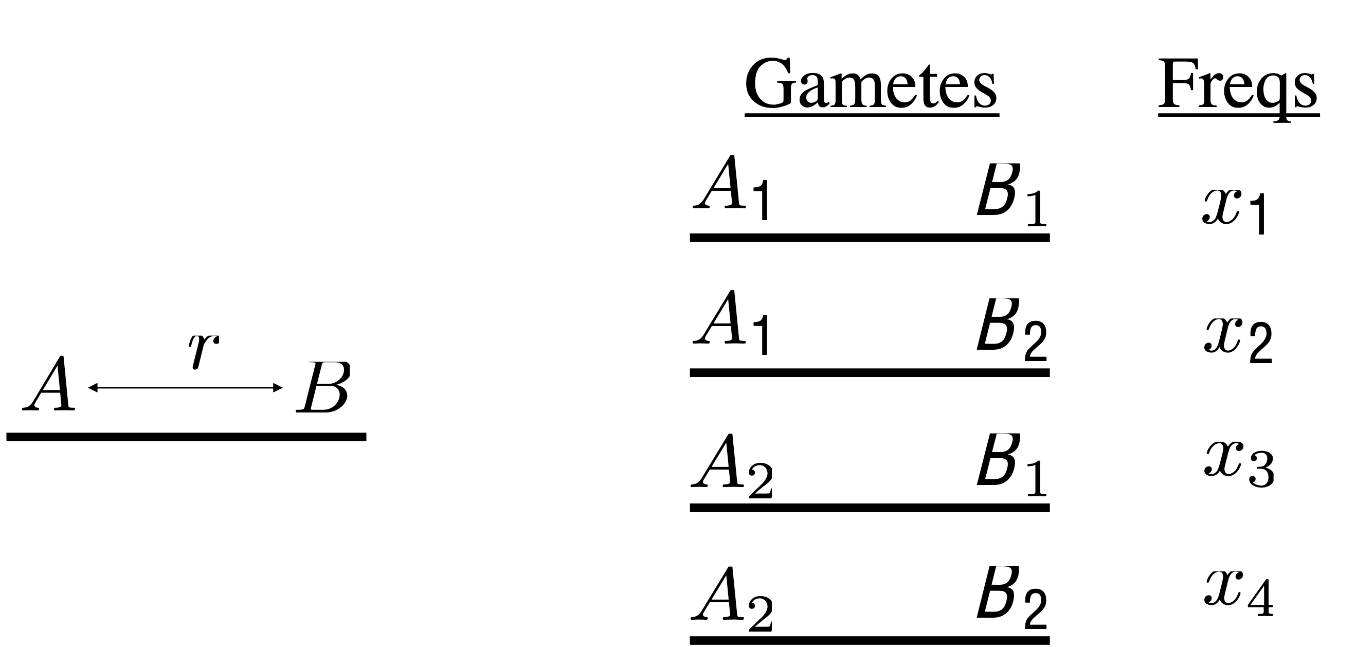
Fig. 12 Two-locus model. The $A$ locus and the $B$ locus have a probability of recombination between them per meiosis of $r$. On the right are given the possible gametes and their associated frequencies¶

With 2 di-allelic loci (2-alleles at each locus) there are 4 possible gametes. We will call their frequencies $X_1,...,X_4$ respectively. Sometimes people draw a distinction between coupling ($A_1B_1$ and $A_2B_2$) and repulsion ($A_1B_2$ and $A_2B_1$) gametes. To my taste this is pretty arbitrary so we’ll try to avoid that terminology although you should know it to be fluent in the language of meiosis. Note that we can write down the frequency of the $A_1$ allele as a function of the gamete frequencies, $p_1 = x_1 + x_2$. It follows than that the frequency of the $B_1$ allele is $p_2 = x_1 + x_3$.

Now lets watch how gamete frequencies change generation to generation as a result of recombination. It’s good to note at the outset of this analysis that recombination only changes gamete frequencies; it does not change allele frequencies. If this point isn’t clear, prove it to yourself by doing a simple cross. After one round of meiosis the frequency of the $A_1B_1$ gamete, $x_1'$ is

\[\begin{aligned} x_1' = (1-r)x_1 + rp_1p_2. \end{aligned}\]

There are two ways to get an $A_1B_1$ allele in the next generation, either it was a recombinant or it was not. The probability that our chosen gamete was not a recombinant is $(1-r)$, so the joint probability of selecting a gamete that was not a recombinant and it being an $A_1B_1$ gamete is simply $(1-r)x_1$. The second way to get an $A_1B_1$ gamete is if it were a recombinant between a gamete carrying an $A_1$ allele (probability $p_1$) and a gamete carrying $B_1$ allele (probability $p_2$). The total probability of this event is $rp_1p_2$ because through recombination we can treat the two loci as independent. These are the two terms of our equation.

Now lets do what comes naturally. The change in frequency of the $A_1B_1$ gamete due to recombination, $\Delta_rx_1$ is

\[\begin{split}\begin{aligned} \Delta_rx_1 & = & x_1' - x_1 \\ \Delta_rx_1 & = & -r(x_1-p_1p_2) \end{aligned}\end{split}\]

The coefficient of $r$ here leads us to the definition of linkage disequilibrium

\[\begin{aligned} D = x_1 - p_1p_2. \end{aligned}\]

$D$ is a measure of the difference in the frequency of the $A_1B_1$ gamete, $x_1$, and what you would expect its frequency to be if alleles were independent (i.e. followed Mendel’s second law). That is to say that if there was no genetic linkage of the $A$ and $B$ locus, we would expect $x_1$ to equal the product of the frequencies of $A_1$ and $B_1$. We can then re-write the change in $x_1$ as a function of $D$,

\[\begin{aligned} \Delta_rx_1= -rD. \end{aligned}\]

Setting $\Delta_rx_1 = 0$ we can find the equilibrium gamete frequency $\hat{x_1}$

\[\begin{aligned} \hat{x_1} = p_1p_2. \end{aligned}\]

This means that at equilibrium there is no linkage disequilibrium between loci, so that gamete frequencies can be predicted from allele frequencies. Thus recombination acts to destroy LD at a rate proportional to the recombination rate between loci. Now step back and think about this- should I see more or less LD between loci that are on distant portions of chromosomes?

Next let’s turn our attention to how $D$ itself changes generation to generation. All we are going to do is plugin our $p_1p_2 + D = x_1$ and recognize that allele frequencies don’t change between generations. This yields

\[\begin{split}\begin{aligned} p'_1p'_2 + D' & = & (1-r)(p_1p_2+D) +rp_1p_2 \\ D'& = & (1-r)D \end{aligned}\end{split}\]

This expression leads intuitively to the difference expression which capture the decay in LD due to recombination

\[\begin{aligned} D_t = (1-r)^tD \end{aligned}\]

and the change in D in any generation due to recombination is

\[\begin{aligned} \Delta_rD=-rD. \end{aligned}\]

So recombination whittles away at allelic associations until there are none left. This decay occurs both across generations (i.e. time) and across what we call genetic distance. Genetic distance refers to the amount of recombination between any two loci- so loci that have more recombination between them should have less allelic association (i.e. lower levels of LD).

Linked Selection¶

We now know a little bit about the dynamics of linked loci under the influence of recombination. What happens when other forces operate? In particular let’s ask the question, how should selection at a linked locus be felt by a neutral locus nearby? We are going to look at the effect of linked selection from two perspectives- it’s deterministic influence on linked variation (genetic hitchhiking) , and it’s stochastic influence on allele frequencies (genetic draft).

Genetic Hitchhiking¶

Adaptation at the molecular level is characterized by beneficial mutations rising to high frequency and eventually fixing in a populations. We call a single iteration of this process a selective sweep. As our beneficial mutation is rising in frequency in the population, it will carry with it its linked genetic background. This process means that variation will be reduced surrounding our beneficial mutation. In the case of no recombination, all variation on the chromosome will be removed from the population. In the case of intermediate levels of recombination, genetic hitchhiking will lead to a local reduction in polymorphism surrounding the beneficial mutation. Thus genetic hitchhiking can be considered to deterministically decrease variation linked to a selective sweep. What do you think this would mean for regions of the genome with lower versus higher levels of recombination?

Genetic Draft¶

In Gillespie’s genetic draft model we focus attention away from the full two locus dynamics of our system and instead concentrate on what happens at a neutral locus linked to a locus undergoing occasional selective sweeps. In this way we can collapse down the dynamics of a two locus system to a one locus perspective.

We begin by following allele frequency change at a neutral locus that is linked to a locus which is undergoing a selective sweep. If sweeps are the only force changing allele frequencies in our population (i.e. an infinite population size) then after a sweep occurs at our neutral locus of interest the frequency of the $A_1$ allele at the neutral locus is

\[\begin{split}\begin{aligned} p' = \left\{ \begin{array}{ll} 1 & \quad \mbox{with probability $p$}\\ 0 & \quad \mbox{with probability $1 - p$}\\ \end{array} \right. \end{aligned}\end{split}\]

where $p'$ goes to 1 if it is linked to the beneficial mutation (i.e. it fixes) or 0 if it is not so lucky. The probability of each of those events is simply the chance the beneficial allele falls on each of the backgrounds.

Note

An important quantity in probability is the expected value of a random variable. The expected value (sometimes called the expectation), tells us what the average outcome of our probabilistic event should be. Formally, if we have a discrete random variable $x$ (e.g. the outcome of throwing a 6-sided die), then we write the expected value of $x$ as

\[\begin{aligned} E\{x\} = \sum_i x_i \times p_i \end{aligned}\]

where the $x_i$s are the possible outcomes of the probability experiment (e.g. 1, 2, 3, etc in our dice toss) and the $p_i$s are the probabilities associated with each event.

Let’s write down the expected value of a random variable which represents one toss of a 6-sided die next. First we will make a table of the possible outcomes and their associated probabilities

outcome ($x_i$)	probability of outcome ($p_i$)
$1$	$\frac{1}{6}$
$2$	$\frac{1}{6}$
$3$	$\frac{1}{6}$
$4$	$\frac{1}{6}$
$5$	$\frac{1}{6}$
$6$	$\frac{1}{6}$

So we can see that each of the possible outcomes of tossing our die is equally likely. Okay, next let’s compute the expected value of $x$, our random variable that will represent a toss of the die

\[\begin{aligned} E\{x\} = \sum_i x_i \times p_i = (1 \times \frac{1}{6}) + (2 \times \frac{1}{6}) + (3 \times \frac{1}{6}) + (4 \times \frac{1}{6}) + (5 \times \frac{1}{6}) + (6 \times \frac{1}{6}) = 3.5 \end{aligned}\]

so the expected value of a single coin toss is 3.5. Does this make sense to you? We will be applying this idea to our study of population genetics when allele frequency itself is stochastic.

Another example that is fun to do– winning the Mega Millions lottery. The probability of winning the Mega Millions is $1$ in $302,575,350$ or approximately $3.3 \times 10^{-9}$. Let’s imagine the jackpot is worth $100 million dollars ($10^8$ USD) and that a ticket costs $1. What’s the expected value of playing the lottery?

outcome ($x_i$)	probability of outcome ($p_i$)
$10^8$ dollars (I win!)	$ 3.3 \times 10^{-9} $
$-1$ dollars (I lose)	$ 1 - (3.3 \times 10^{-9}) $

Okay so that’s the table, and the expected value is

\[\begin{aligned} E\{x\} = \sum_i x_i \times p_i = (10^8 \times 3.3 \times 10^{-9}) + (-1 \times (1-(3.3 \times 10^{-9}))) = -0.67 \end{aligned}\]

So your expected value from playing the lottery is negative. This means that you should expect to lose money!!

Next let’s find the expected value of the allele frequency in the next generation,

\[\begin{aligned} E\{p'\} = ( 1 \times p) + ( 0 \times (1-p)) = p \end{aligned}\]

so on average we expect no change in allele frequency due to genetic draft (i.e. linked selected sweeps).

We can do exactly the same thing but now allow there to be a probably of no sweep occurring in generation. Call the probability of a sweep per generation

\[\begin{split}\begin{aligned} Prob(sweep) = \rho \\ \end{aligned}\end{split}\]

now let’s fix up our model below to allow fo the possibility of no sweep in a given generation.

\[\begin{split}\begin{aligned} p' = \left\{ \begin{array}{ll} p & \quad \mbox{with probability $(1-\rho)$}\\ 1 & \quad \mbox{with probability $\rho p$}\\ 0 & \quad \mbox{with probability $\rho(1 - p)$}\\ \end{array} \right. \end{aligned}\end{split}\]

In words, we are saying that there are three possibilities under this model for the new allele frequency– if there is no sweep it remains unchanged, if there is a sweep and our allele is the one that fixes then $p$ goes to $1$, or the last possibility is that there is a sweep and the other allele fixes so $p$ goes to 0.

So now let’s write down the expected value of $p'$ in this new model

\[\begin{split}\begin{aligned} E\{p'\} & = & (p \times (1-\rho)) + (1 \times \rho p) + (0 \times \rho (1-p))\\ E\{p'\} & = & p \end{aligned}\end{split}\]

So again we end up in a situation where on average there is no change in allele frequency. Just like drift!

Finally at equilibrium, Gillespie was able to work out what heterozygosity should look like when mutations and sweeps are occurring

\[\begin{aligned} \hat{H}_{draft} = \frac{4Nu}{1+4Nu+2N\rho} \end{aligned}\]

Lecture 10: Evolution as a combination of forces

Lecture 12: Molecular Evolution

outcome (\(x_i\))	probability of outcome (\(p_i\))
\(1\)	\(\frac{1}{6}\)
\(2\)	\(\frac{1}{6}\)
\(3\)	\(\frac{1}{6}\)
\(4\)	\(\frac{1}{6}\)
\(5\)	\(\frac{1}{6}\)
\(6\)	\(\frac{1}{6}\)

outcome (\(x_i\))	probability of outcome (\(p_i\))
\(10^8\) dollars (I win!)	\( 3.3 \times 10^{-9} \)
\(-1\) dollars (I lose)	\( 1 - (3.3 \times 10^{-9}) \)

Bio 380-- Evolutionary Biology