
Lecture 19: Phylogenetics II: Methods and Maximum-likelihood
Contents
Lecture 19: Phylogenetics II: Methods and Maximum-likelihood
Molecular biology has revolutionized the field of systematics. DNA evolves by mutations being incorporated in the DNA and fixed in populations. This will lead to divergence of DNA sequences in different species. Although diverged, we can refer to two DNA sequences as homologous (just as we would for any morphological trait such as forelimbs). Nicely demonstrates descent with modification as a definition of evolution. For this reason, DNA should be an excellent tool for inferring phylogenies: large number of homologous characters that should be (maybe) less subject to convergent evolution than other characters that might lead to a confusion of grade and clade.
Measuring Evolutionary distance
To estimate phylogenies we first must estimate how much sequence divergence there has been between the various taxa we want to study. Several methods: direct sequencing. Elegant molecular methods available, a lot of work but provides lots of data. Each nucleotide position is a character and the actual nucleotide that is present at that site is the character state.
A character can be phylogenetically informative when nucleotide changes are shared by two or more taxa. A character can be phylogenetically uninformative when all nucleotides are the same among taxa, or when only a single taxon has a different nucleotide.
A less direct method of determining sequence divergence is by restriction enzyme mapping. These are enzymes that recognize specific sequences in the DNA and cut the DNA strands. Depending on the location of restriction recognition sites in the DNA, DNA fragments of various lengths will be generated by the restriction enzyme digest resulting in a restriction fragment pattern. One can also determine where various restriction enzymes cut a given piece of DNA and draw up a restriction map of the stretch of DNA. The extent to which two restriction maps (or restriction fragment patterns) are similar serves as an estimator of sequence similarity (or difference). Restriction enzymes will recognize only a fraction of the entire DNA sequence, so one will not know all the differences between two stretches of DNA. The data serve as an estimate and because it usually involved less work can be done on many individuals. DNA-DNA hybridization is another indirect way of obtaining estimates of DNA sequence divergence between two taxa. DNA strands are melted apart at high temperature and allowed to “reanneal” in the presence of the DNA of another species. One species’ DNA has been labeled with a radioactive nucleotide. This form heteroduplex DNA. The heteroduplex DNA is gradually heated and the amount of single stranded DNA that has “melted” apart is determined by the amount of radioactive label that is counted in each fraction collected from the various temperature steps. Very similar DNA will melt at a high temperature and heteroduplexes between diverged DNAs will melt at a lower temperature. Sequence divergence is proportional to melting temperature.
Phenetic approaches: DNA hybridization, sequence divergence from sequencing, restriction patterns or restriction maps. In each case the data would be in the form of a single number indication the similarity or difference between the DNAs of each pair of species in the study.
Cladistic approaches: direct sequencing, restriction maps and restriction fragments (fragments less desirable). In each case one would look for shared derived character states (nucleotide, restriction recognition site) among taxa. With restriction sites shared loss is unreliable as a uniting character because the nucleotide change could have occurred anywhere in the recognition sequence. Like refrigerator/pizza/invertebrate example.
A note on phylogeny
It’s good just to clear up a few definitions at this point that could aid your understanding of cladistic species concepts. The big three are monophyly, paraphyly, and polyphyly:
Monophyletic group: a group that consists of an ancestor and all of its descendants
Paraphyletic group: a group that contains the most recent common ancestor (MRCA) but not all its descendants
Polyphyletic group: a group whose MRCA is not a member of the group
The only one of these three that is meaningful biologically is a monophyletic group.
Molecular approaches to systematics for us to think about the rates of molecular evolution. If DNA or proteins evolved at a constant rate in all species, then one could use estimates of sequence divergence to build very reliable phylogenies. If there was a molecular clock we could determine the “true phylogeny”. Fact is, there is no one molecular clock.
Different proteins and DNA sequences evolve at different rates. Why? Different functional constraints. Different proteins do different things and some can do their structural or functional job with any of several different amino acids at many of the positions (fibrinopeptides). Other proteins will not function properly with “any” amino acid changes (histones: two amino acid differences between peas and cows!). Intron sequences less constrained than coding exon sequences, and hence introns tend to diverge faster than exons. Synonymous sites evolve faster than non-synonymous sites, again due to different functional constraints (i.e., some form of selection against “incorrect” sequences). Nuclear DNA tends to evolve slower than mitochondrial DNA (in vertebrates). Unit evolutionary period: time required to observe a given unit of divergence. A 1% divergence of vertebrate mitochondrial DNA takes about 250,000 to 500,000 years.
What gene do I use??: Depends on the taxa you are studying and the amount of divergence among them. Histones good for “macrosystematics”, fibrinopeptides, mtDNA good for “microsystematics” or population level phylogenies.
Note problems with tree building from data: unequal rates and convergence.
As if the choice of gene/protein were not a problem. What if different lineages evolve at different rates? Test for this with the relative rate test. Compare the paths from two different taxa to a third taxon. If the paths are the same: taxa are evolving at the same rate; if not: different rates. Extreme rate fluctuations are a problem; slight ones are not as they would not lead to regrouping taxa (depending on how “slight” is defined)
Convergence over long stretches of DNA is unlikely, although it has been reported for lysozyme. Another kind of “convergence” can occur due to the limited number of character states in DNA. Back mutations: e.g. A changes to T, T changes to C and C changes back to A. Could occur in one step or many. Maximal random divergence: 25% similarity
Nonetheless molecular tools have allowed major leaps in our understanding of biological diversity: Bacterial evolution: three kingdoms, not five; Endosymbiont hypothesis, essentially proven; AIDS virus: rapid evolution is good for the virus, bad for us.
Maximum Likelihood
The modern methodology that allows us to deal with the problems of back mutation, rate variation, etc. in a rigorous framework is known as Maximum Likelihood phylogenetics (ML). ML was a technique for estimating parameters in probability models that was introduced in the early part of the 20th century by none other then our man, R. A. Fisher. ML estimation is very easy to understand and implement, and very powerful in the results it produces. The idea behind ML is that the value of some parameter that makes our data most probable (likely) is desirable. Simple right?
Lets examine the ML principle using a simple toy example. Imagine that a friend passes you a coin that he says is fair (i.e. prob. of heads = 0.5) and you want to test if indeed it is fair. You flip the coin 10 times and get 8 heads. A coin flipping experiment like this follows a binomial distribution. Let’s call the probability of getting a heads on a single flip, \(p\). If you flip a coin \(n\) times the probability of getting heads \(k\) times is
The probability of getting 8 heads is
Now lets estimate the parameter \(p\) in our model above by maximum likelihood. Remember that a “fair” coin has \(p=0.5\) corresponding to a \(1/2\) chance of getting heads. We say that the likelihood function of the parameter is just the probability of getting our data given that parameter. That is
All we have to do now is maximize the likelihood function and we will get our maximum likelihood estimate (MLE) of our parameter. This can of course be done analytically by writing down a closed form solution of the MLE, but this can’t be achieved in all cases. This is where computers and numerical methods come in- all we need to do is be able to calculate the likelihood function (which isn’t always the case) and we can get an MLE of our favorite parameters. In our present example let’s look at the likelihood function as a function of \(p\) in Fig. 17
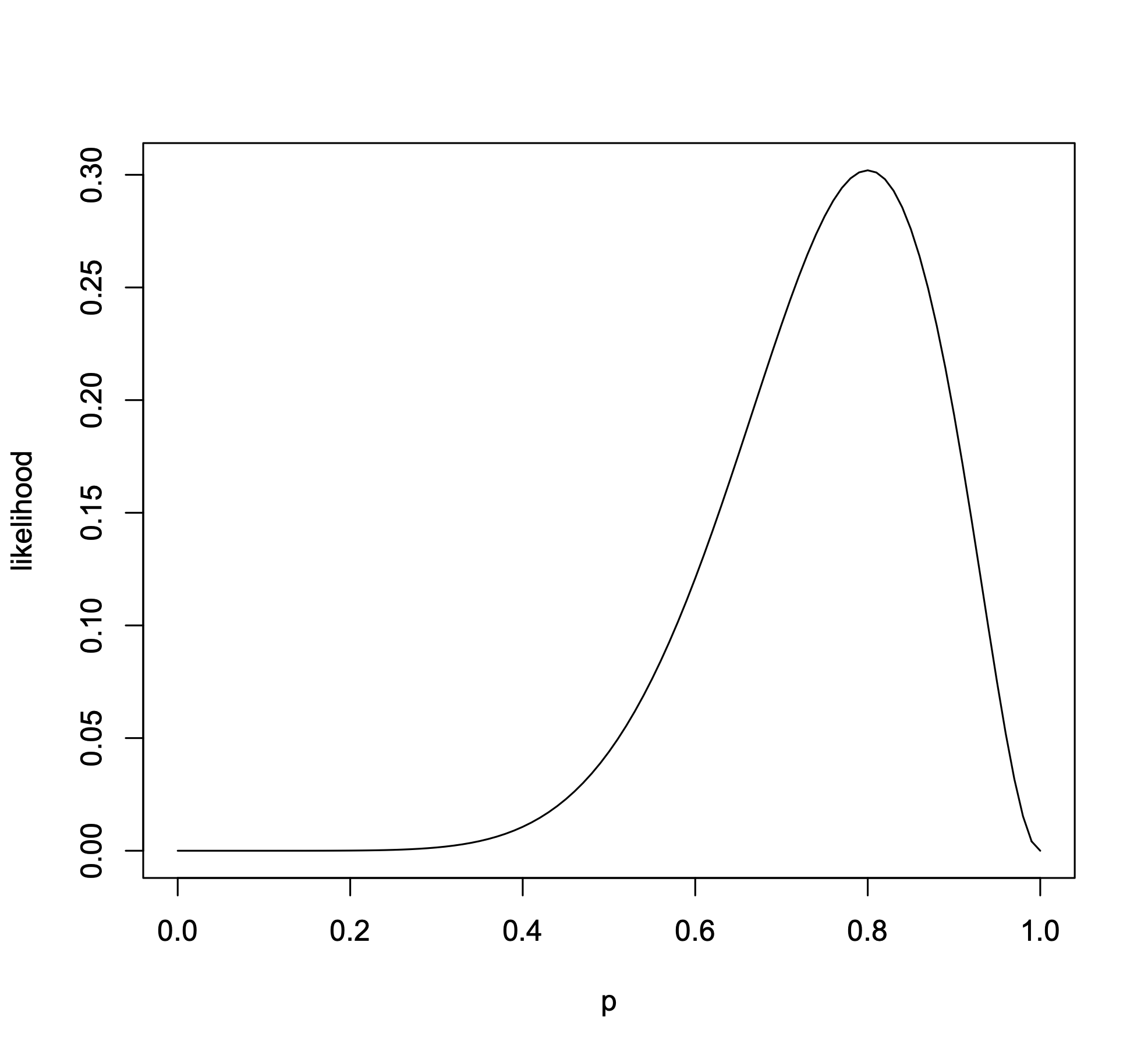
Fig. 17 The likelihood function of our coin flipping example. The data are binomially distributed with \(x=8\) being our observed data
In general ML estimation works by writing down the likelihood function of some parameter, that is
and then maximizing that function to get ML estimates of our parameters. Simple no?
Maximum Likelihood Phylogenetics
In phylogenetics the likelihood calculation we are interested in is \(Prob(\mbox{data} | \mbox{tree})\). Notice that the tree is actually composed of two parts, the topology (who’s related to who and in what sequence) and the set of branch lengths. Consider the tree in Fig. 18. Here the \(x^is\) represent the character states and the \(t_is\) represent branch lengths. You’ll notice too that we’ve labeled character states at interior nodes to represent ancestral (unobserved) conditions.
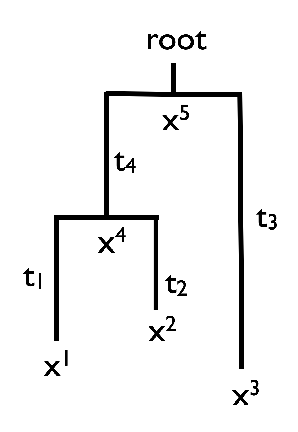
Fig. 18 A 4 taxon rooted tree. Here the \(x^is\) represent the character states and the \(t_is\) represent branch lengths.
Now lets assume for a second that we can write down the probability of going from state \(x^j\) to state \(x^i\) in time \(t\)
We will look into the details of this in a second. With this assumption we are now in a position to write down the probability of the data given our tree (i.e. the likelihood). This probability is simply the probabilities of what happens on each branch of the tree multiplied together. That is
where \(P(x^5)\) represents the probability of being in state \(x^5\) at the root. In general we don’t know the ancestral states, so we will sum over all of there possibilities. This is a tremendous leap forward in our phylogenetic thinking- rather than assume some ancestral condition as in parsimony we will now formally sum across all possibilities. This is a huge difference philosophically.
For a moment lets call the complete set of observed data \(x^\cdot\) and the complete set of branch lengths \(t_\cdot\). The ML phylogenetic problem can then be written simply as \(P(x^\cdot | T, t_\cdot)\). Finding an ML tree then requires two parts: 1) a search over different tree topologies \(T\) and 2) optimization of branch lengths given a tree. The former is very difficult given how the number of trees explodes with the number of taxa. The latter is simpler.
Likelihood of two taxon tree
To illustrate the likelihood calculation lets turn our attention to a very simple tree- a two taxa rooted tree (Fig. 19). Let’s imagine that we’ve collected some sequence data from two taxa. Those sequences might be
\(\begin{aligned} \mbox{CCGC}\\ \mbox{CGGG} \end{aligned}\)
and we want to write down the probability of the data at the \(k\)th site given our tree
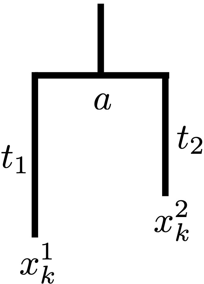
Fig. 19 A 2 taxon rooted tree. \(a\) represents the ancestral state.
\(q_a\) here represents the probability of drawing state \(a\) from the root distribution. We assume that this is actually the stationary distribution of the substitution matrix– more in a sec. So this probability is the joint probability of choosing \(a\) and then substituting from \(a\) to state \(x^1\) at site k along lineage \(t_1\) and also substituting from \(a\) to state \(x^2\) along lineage \(t_2\). As we don’t know what the ancestral state was (can’t observe it) we will sum across all possible ancestral states to arrive at our likelihood
Again, this summing up over ancestral states is huge! If we had \(n\) sites in our sequence alignment we can write down the full likelihood of our data by assuming independence among sites and thus multiplying likelihoods. That is
We’re halfway there to full blown ML phylogenetics
Probabilistic models of DNA evolution
The second half left to tackle is the probability of substitution in some unit time, \(Prob(x^i|x^j,t)\). There is a rich tradition of coming up with models like this. The state of the art technology uses continuous time Markov models to model the substitution process. Simplest model of this form is the Jukes-Cantor (1969) model which assumes all substitutions occur at a symmetric rate. The transition matrix, \(P\), for this model is given by
You’ll notice that the values on the diagonal all are equal to \(1-e\alpha\). This is dictated by the Markov principle which states that the sum of all rows must equal one– i.e. the probabilities of all transitions from a state must equal one. The other thing to notice is that the transition probabilities between each state are symmetric- not a very realistic model, but it will do for now.
After a little bit of linear algebra which we will skip over we can write down the the equilibrium substitution probabilities
Basically there are only two probabilities we are worried about- the probability that the states are the same, and the probability that the states are different. Everything else is symmetric and thus equal to one of these to probabilities. Let’s then move on to use this Jukes-Cantor model with our two taxon tree data.
Likelihood of two taxon tree with substitutions
The first order of business is to use the expressions from the Jukes-Cantor Model to write down the probabilities of having the same and different sequence at each site in our tree. The probability of seq1 being a C and seq2 being a C given our tree is
This will be true for all pairs of different nucleotides which are different from one another due to the assumptions of our nucleotide substitution model. The probability of seq1 being a C and seq2 being a G given our tree is
and again this will be true for all pairs of mismatched nucleotides.
Full likelihood then is product of independent site probabilities
I’d encourage the reader to go figure out this probability numerically. That’s all there is basically to ML phylogenetics. Once you understand the principle of summing over ancestral character states all you need is a decent way to algorithm to calculate the tree probabilities (think dynamic programming) and a decent substitution model and your off!