
Lecture 7: Natural Selection II: Population Genetics
Contents
Lecture 7: Natural Selection II: Population Genetics
Natural Selection
Natural selection is arguably the single most important evolutionary force. The products of natural selection surround us- our biochemical sophistication, our finely tuned genetic systems, the incredible fit of organisms to their environments- however witnessing the change brought about by natural selection is nearly impossible in the human life time. Evolutionary change is simple too slow for the human observer. Thus we turn our attention to mathematical models of natural selection which when poked and prodded, will reveal much of the subtle nuance of evolution via natural selection.
The basic model of viability selection
We will again turn to our simplistic model of diploid, randomly mating hermaphrodites to study the fundementals of natural selection. Keep in mind that this model is for convenience, we can also study more realistic models (dioecious species, non-random mating, etc.), however our basic model has nearly all of the same features as more realistic models and is readily tackled mathematically.
Our little hermaphrodites have a simple life cycle, randomly chosen gametes fuse to form zygotes, then these zygotes must survive to adulthood, adults must then be fertile to reproduce and produce offspring. You’ll notice that we’ve added two parts to our simple Hardy-Weinberg model, namely survivorship and fecundity. If the \(A_iA_i\) genotype has genotype-specific survivorship \(l_{ii}\) and fecundity \(m_{ii}\), then the life cycle outlined above can be represented as Genotype \(\rightarrow\) zygote \(\rightarrow\) \(l_{ii}\rightarrow\) adult \(\rightarrow\) \(m_{ii} \rightarrow\) offspring. We are now ready to understand how survivorship and fecundity differences between genotypes can lead to differences in genotype frequencies, outlined in Table 1.
Genotype \(\rightarrow\) |
zygote \(\rightarrow\) |
\(l_{ii}\rightarrow\) |
adult \(\rightarrow\) |
\(m_{ii} \rightarrow\) |
offspring |
|---|---|---|---|---|---|
\(A_1A_1\) |
\(p^2\) |
\(p^2l_{11}\) |
\(p^2m_{11}l_{11}\) |
||
\(A_1A_2\) |
\(2pq\) |
\(2pql_{12}\) |
\(2pqm_{12}l_{12}\) |
||
\(A_2A_2\) |
\(q^2\) |
\(q^2l_{22}\) |
\(q^2m_{22}l_{22}\) |
For the most part, we will consider the probability of representation to be the joint probability of surviving to adulthood and reproducing. This leads to our first formal definition of viability or absolute fitness. Let the viabilities of the \(A_1A_1\), \(A_1A_2\), and \(A_2A_2\) genotypes be \(w_{11}\),\(w_{12}\), and \(w_{22}\) respectively. Further let these viabilities be the joint probability of survival and reproduction such that \(w_{ii} = l_{ii} \times m_{ii}\). Thus we can see that the frequency of a genotype after a round of selection (i.e. in the next generation after selection has occured) is proportional to the frequency of a genotype before selection times the viability of that genotype. For example, the frequency of the \(A_1A_2\) genotype after a round of selection is proportional \(2pqw_{12}\).
Next we are interested in figuring out the relative frequencies of genotypes after a round of selection. To do this we require some constant that will allow genotype frequencies after selection to sum to one. This is where the average fitness of a population comes in as we looked at in lecture.
Genotype: |
\(A_1A_1\) |
\(A_1A_2\) |
\(A_2A_2\) |
|---|---|---|---|
Frequency before selection: |
\(p^2\) |
\(2pq\) |
\(q^2\) |
Viability: |
\(w_{11}\) |
\(w_{12}\) |
\(w_{22}\) |
Frequency after selection: |
\(p^2w_{11}/\bar{w}\) |
\(2pqw_{12}/\bar{w}\) |
\(q^2w_{22}/\bar{w}\) |
The constant, \(\bar{w}\), is equal to
First notice that \(\bar{w}\) represents the frequency weighted average fitness of our population. Next also note that this didn’t pop out of thin air but is instead chosen such that
thus making sure that we can calculate relative frequencies of genotypes after selection. Examine this equation and the table closely- what you’ll notice is that what is important in determining the frequency of a genotype in the next generation is not it’s viability per se, but instead its viability relative to the average viability (fitness) of the population.
Unlike under Hardy-Weinberg dynamics, natural selection can change allele frequencies. If we focus attention on the \(A_1\) allele we can write down its frequency after a round of selection \(p'\) as
Ask yourself this question: why is the second term in the numerator \(pqw_{12}\) and not \(2pqw_{12}\)? Got it? You guys are all gonna be great little population geneticists one day!
The next order of business is to write down the change in allele frequency due to selection in a single generation. That is \(\Delta_sp = p' - p\),
which after some algebraic fiddling yields
We can now see how selection alone should change allele frequencies as a function of genotypic viability. This result is certainly one of the most important results in all of population genetics and evolution.
Relative Fitness
As we noticed earlier and made plain in equation 6, the change in allele frequency due to selection is dependent not just on the viability of a genotype alone, but instead on the viability of that genotype relative to the average viability of the population. This leads us to the distinction between absolute fitness and relative fitness. Absolute fitness can be understood as the probability of a genotype surviving to adulthood and then reproducing. That’s all well and good, but when we are interested in evolution the only thing that counts is how well that genotype performs in relation to others in its population. Thus we will define relative fitness to be the viability of a genotype standardized by the maximum genotypic viability. This won’t change any of the mechanics that we just derived, but instead will make them clearer to understand. Consider the following table
Genotype: |
\(A_1A_1\) |
\(A_1A_2\) |
\(A_2A_2\) |
|---|---|---|---|
Viability: |
\(w_{11}\) |
\(w_{12}\) |
\(w_{22}\) |
Relative viability: |
1 |
\(w_{12}/w_{11}\) |
\(w_{22}/w_{11}\) |
So far we’ve been calling the \(w_{ij}\)’s viabilities- in the business they are more commonly referred to as the absolute fitnesses of the individual genotypes. One we have normalized the \(w_{ij}\)’s by the most fit genotype in the population we end up with relative fitness values for each genotype. The common notation for relative fitness is
Genotype: |
\(A_1A_1\) |
\(A_1A_2\) |
\(A_2A_2\) |
|---|---|---|---|
Relative Fitness: |
\(1\) |
\(1 -hs\) |
\(1 - s\) |
where \(1-hs = w_{12}/w_{11}\) and \(1-s = w_{22}/w_{11}\). The parameter \(s\) is called the selection coefficient. It is a measure of how fit the \(A_2A_2\) genotype is relative to the \(A_1A_1\) genotype. In this setting, if the selection coefficient is positive then the \(A_2A_2\) genotype is less fit than the \(A_1A_1\) genotype. Conversely if the selection coefficient is negative, then the \(A_2A_2\) genotype is more fit. We’ll always assume that \(0\leq s \leq1\) in this class, but notice that all of this notation is really just arbitrary. We’re simply assuming that the \(A_1\) allele is generally the confers some fitness benefit to the genotype.
What about the \(h\) parameter? This parameter is sometimes called the heterozygous effect, as it measures the difference in fitness between the heterozygotes and the two homozygote genotypes. In essence though, \(h\) really defines the dominance relations between the 2 alleles at our locus. This is shown in the following table
\(h\) |
dominance |
|---|---|
\(h = 0\) |
\(A_1\) dominant, \(A_2\) recessive |
\(h = 1\) |
\(A_2\) dominant, \(A_1\) recessive |
\(0 < h < 1\) |
co-dominance |
\(h < 0\) |
overdominance |
\(h > 1\) |
underdominance |
Generally in genetics we are interested in the cases of co-dominance, overdominance, and underdominance. The complete dominance setting, although seen in morphological traits often, is generally unrealistic for most genetic situations. Why would this be?
We are now fully armed to rewrite equation 6 in terms of relative fitness. This will lead to a much more provocative construction of this same equation. So the change in frequency of the \(A_1\) allele due to selection is then
and we can write down the population mean fitness as
The only thing I’ve done to get these formulations is replace \(w_{11}, w_{12}\) and \(w_{22}\) with \(1,1-hs\), and \(1-s\) respectively.
Flavors of selection
We talk generally about 3 kinds of selection: directional selection (as occurs with co-dominance), balancing selection (overdominance), and disruptive selection (underdominance). We have already looked at what these types of selection do at the phenotypic level during lecture. What are the effects of these distinct flavors of selection on allele frequencies? To examine this we will examine the fate of the \(A_1\) allele in a population, given values for the parameters \(h\) and \(s\) and assuming some initial frequency of the \(A_1\) allele.
Directional selection
Directional selection is perhaps the most familiar form of selection. This is the kind of selection that Charles Darwin had in mind when he wrote about evolution by natural selection. Directional selection occurs in the case of incomplete dominance (\(0 \leq h \leq 1\)). In this case the frequency of the \(A_1\) allele, \(p\), should always increase, or seen another way \(\Delta_sp > 0\). Fig. 6 plots \(\Delta_sp\) as a function of \(p\). As an exercise, plot how \(p\) changes from generation to generation. Does the \(A_1\) allele always fix (i.e. \(\rightarrow 1\)) in the population?
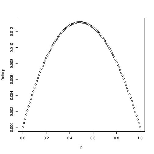
Fig. 6 Directional selection. Shown is the change in allele frequency \(\Delta_sp\) as a function of allele frequency \(p\). In this case \(h=0.5\) and \(s=0.1\)
One thing to notice- the change in allele frequency is slowest when there is little genetic variation in the population (i.e. when \(p\) is close to zero or one). Be sure that you can explain to yourself why this is.
Balancing selection
The second kind of selection occurs when there is overdominance (i.e. \(h < 0\)). Unlike directional selection, balancing selection leads to the maintenance of variation within a population. That is to say the the allele frequency of the \(A_1\) allele will approach some equilibrium value \(\hat{p}\) independent of initial frequency. We will plot this again graphically by looking at the change in allele frequency as a function of allele frequency.
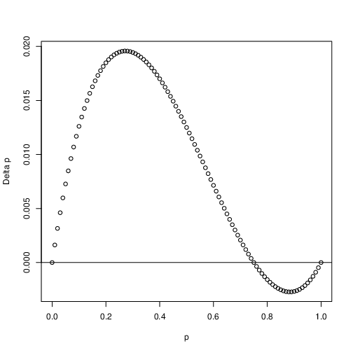
Fig. 7 Balancing selection. Shown is the change in allele frequency \(\Delta_sp\) as a function of allele frequency \(p\). In this case \(h=-0.5\) and \(s=0.1\)
.
Let’s look closely at Fig. 7. Notice that when \(p\) is close to zero \(\Delta_sp > 0\) and thus allele frequency will increase when rare. Conversely when \(p\) is close to one \(\Delta_sp < 0\) and allele frequency will decrease. Where is the stable equilibrium in this figure? It is left to the reader to find this equilibrium point. You can do so by setting \(\Delta_sp = 0\) and solving for \(\hat{p}\).
Disruptive selection
The last kind of selection we will look at is disruptive selection. This occurs with overdominance, \(h > 1\). Fig. 8 again graphs \(\Delta_sp\) as a function of \(p\). What’s curious in this case is that \(p\) will decrease when rare and increase when common in the population. This means that if \(p\) is less than \(\hat{p}\) the allele will be lost, and if \(p>\hat{p}\) it will fix. Thus \(\hat{p}\) is an unstable equilibrium. If by some strange circumstance \(p = \hat{p}\) allele frequencies won’t change at all! Needless to say underdominance is rare in nature…
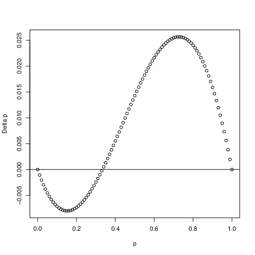
Fig. 8 Disruptive selection. Shown is the change in allele frequency \(\Delta_sp\) as a function of allele frequency \(p\). In this case \(h=2\) and \(s=0.1\)
.