Lecture 8: Mutation, Migration, with and without selection

Mutation and Evolution

Previously we learned about how selection can change the frequencies of alleles and genotypes in populations. Selection typically eliminates variation from within populations. (The general exception to this claim is with the class of selection models we have called “balancing” selection where alleles are maintained in the population by overdominance, habitat-specific selection, or frequency dependent selection). If selection removes variation, soon there will be no more variation for selection to act on, and evolution will grind to a halt, right? This might be true if it were not for the reality of mutation which will restore genetic variation eliminated by selection. Thus, mutations are the fundamental raw material of evolution.

The basic model of mutation that we will study is one way mutation. This is when one allele through mutation can turn into another such that

\[\begin{aligned} A_1 \stackrel{u}\longrightarrow A_2 \end{aligned}\]

\(u\) here represents the mutation rate, the probability that a mutation from \(A_1\) to \(A_2\) occurs during a meiosis.

It should be obvious that mutation will change allele frequencies. This is true because there is a constant flux from \(A_1\) to \(A_2\) purely as a result of this mutation process. We can study the change in allele frequency due to mutation in a very similar way to how we studied the change in allele frequency due to selection. Consider a population with frequency of the \(A_1\) allele \(p\). In the next generation, after a round of mutation, each \(A_1\) allele must have been \(A_1\) in the current generation and it must not have mutated. That is

\[\begin{aligned} p' = p (1-u). \end{aligned}\]

Now let’s turn our attention to the change in allele frequency in one generation due to mutation as we did previously for selection

(3)\[\begin{split}\begin{aligned} \Delta_up &= p' - p \\ &= p(1-u) -p \\ &= -up \end{aligned}\end{split}\]

Notice that our notation– \(\Delta_up\) – emphasizes the source of the change in allele frequency is mutation.

This sort of unidirectional mutation acts to consistently decrease the frequency of the \(A_1\) allele from generation to generation. If we instead were to study two way mutation, the mutational flux would depend on the proportional rates to and from \(A_1\). So mutation, although it is a random process with respect to target, leads to deterministic effects on allele frequencies. Neat huh?

Mutation rates per generation are very very small. In Drosophila, which is one of the best studied animals from the perspective of rates of spontaneous mutation, the mutation rate per generation per nucleotide is on the order of \(10^{-9}\) (Keightley et al. 2014). In humans it’s a bit higher, about \(1.2 \times 10^{-8}\) (remember from Lecture 4), but either way that’s tiny. This means that mutation changes the frequency of alleles at a very slow rate. If we assume that there is sufficiently strong selection against the \(A_2\) allele (i.e. \(w_{11} >> w_{22}\)), then \(A_2\) will be rare and we can further approximate our change in allele frequency due to mutation

(4)\[\begin{split}\begin{aligned} \Delta_up &= -up \\ &= -u + qu \\ &\approx -u, \end{aligned}\end{split}\]

because \(q \approx 0\). So in the case of a deleterious \(A_2\) allele, we can see that the change in allele frequency due to mutation is independent of allele frequencies. This is our first hint that mutation and selection might combine in interesting and important ways.

Mutation-Selection Balance

We can imagine mutation and selection as opposing forces which might come to some equilibrium in terms of the number or frequency of deleterious alleles within a population. To make this concrete think about the human genetic disease cystic fibrosis (CF). CF is a very serious genetic disorder in which a transmembrane protein in lung epithelium cells called CFTR is non-functional. Hundreds, if not thousands of separate mutations in CFTR lead to CF, thus we could imagine that there is a certain, appreciable rate of mutation to CF. If each of these mutations is deleterious (i.e. they cause disease) then over generations they should be selected out of the population. Thus mutation will inject CF mutations into the population, but selection will remove them- can we study this as an equilibrium process?

Our approach will be to study each of our evolutionary forces in isolation, and then combine them to figure out how they interact. Let’s start by considering the change in allele frequency due to selection that we studied in lecture 7, but this time we will approximate it under the assumption that \(q \approx 0\)

(5)\[\begin{split}\begin{aligned} \Delta_sp &= \frac{pqs[ph + q(1-h)]}{\bar{w}} \\ &\approx qhs \end{aligned}\end{split}\]

This approximation works because when \(q \approx 0\), then \(p \approx 1\) and \(\bar{w} \approx 1\), and we can ignore all terms of order \(q^2\).

Now let’s combine the forces of selection and mutation on the change in frequency of \(A_1\) using the approximations we have just derived (equations (4) and (5)). At equilibrium the change in allele frequency due to the combined actions of mutation and selection must equal zero. That is

\[\begin{split}\begin{aligned} 0 &= \Delta_up + \Delta_sp \\ &\approx -u + qhs \end{aligned}\end{split}\]

so the equilibrium frequency of the \(A_2\) allele is

\[\begin{aligned} \hat{q} \approx \frac{u}{hs} \end{aligned}\]

Thus we see that deleterious (e.g. disease) allele frequencies are determined by both the mutation rate to those alleles and their selective effects in heterozygotes. As we saw earlier, new mutations overwhelmingly are found in heterozygous states, so it’s perhaps not surprising that \(h\) should dominate the fate of deleterious alleles.

This equilibrium has a name, mutation-selection balance. Let’s be precise about what it means. At \(\hat{q}\) both forces are still working every single generation- mutation is creating new copies of the deleterious allele and selection is removing copies of it. They’re just doing so at exactly the same rate, so the allele frequency stops changing. That’s why deleterious alleles never go away completely. The population always carries some standing load of them, and how big that load is depends on the ratio of the mutation rate to the strength of selection against heterozygotes.

Problem: Go through the same steps of approximations that we just did to find the Mutation-Selection equilibrium value of mutations which are completely recessive (i.e. \(h = 0\)). This would make a heck of an exam question…

Follow up: Once you’ve got your answer, let’s go back to CF. CF is recessive, and until pretty recently in human history people with CF basically never survived to have kids, so \(s \approx 1\). In people of European ancestry the frequency of CF alleles is something like \(q \approx 0.02\) (about 1 in 25 people carries one). Plug those into your answer and solve for the mutation rate you would need to keep CF at that frequency. How does that compare to the mutation rates we just talked about? If mutation-selection balance can’t explain it, what else might be going on?

Migration and Gene Flow

In population genetics, the term “migration” is really meant to describe gene flow, defined as the movement of alleles from one area (deme, population, region) into another, where they get passed on to the next generation. Gene flow requires some form of dispersal or migration (wind pollination, seed dispersal, birds flying, etc.) but dispersal is not gene flow. Genes must be transferred, not just their carriers. A bird that flies to a new island and dies before breeding has dispersed, but it hasn’t contributed any gene flow at all.

We are going to build a model of gene flow in exactly the same way we studied mutation. Consider two populations, a mainland population and an island population. Each of these populations has the \(A_1\) allele at frequencies \(p_{main}\) and \(p_{island}\) respectively. Assume that gene flow is one way, from mainland to island, and that each generation a proportion \(m\) of the parents in the island population are migrants who just arrived from the mainland. Although I’ve said this is a proportion, also notice that we could consider this a probability interchangeably. After a round of migration, in the island population there are then two sources for alleles, they could be from the island population originally with probability \(1-m\), or they could have migrated from the mainland with probability \(m\). This means that after migration the allele frequency of \(A_1\) in the island population is

\[\begin{aligned} p_{island}' = p_{island}(1-m) + p_{main}m. \end{aligned}\]

Simple enough right? Now let’s do what comes naturally and study the change in allele frequency as a result of migration. Following what we have done in our other analyses,

\[\begin{split}\begin{aligned} \Delta_{m}p_{island} &= p_{island}' - p_{island} \\ &= p_{island}(1-m) + p_{main}m - p_{island} \\ &= m(p_{main} - p_{island}) \end{aligned}\end{split}\]

Beautiful. Now we have a very simple expression for how allele frequencies in the island population should change due to gene flow from the mainland population. This change in allele frequency makes sense- it only depends on the amount of migration and the differences in allele frequencies between the two populations. It’s simple enough to generalize this to multiple populations, or to populations at different distances away from one another, but we won’t cover that here.

Migration and Selection

One of the fundamental observations in biology and natural history is that of local adaptation- populations of organisms adapt to their local surroundings. To be precise, a population is locally adapted when its members have higher fitness in their home environment than members of other populations of the same species do when they’re put there. The classic way to test for this is a reciprocal transplant experiment. Take individuals from two populations, move each into the other’s habitat (and back into their own as a control), and measure how well they survive and reproduce. If each population does best at home, you’ve got local adaptation. Think of populations of plants that live in dry environments that might be better able to handle drought than their conspecifics who live in wet environments. Or think back to the cline in human skin pigmentation from Lecture 4, where populations are adapted to the amount of UV radiation where their ancestors lived. How does this kind of adaptation take place in the face of the homogenizing influence of gene flow? The answer is through the interplay between migration and selection.

We will study this struggle between migration and selection in exactly the same way we have studied the other combinations of forces in this lecture. Consider that some weak allele is wafting over to the other side of the tracks, so to speak, where it does not survive (e.g., fish swimming into New York harbor). There is an evolutionary pressure changing allele frequencies in one direction (into the harbor), and an opposing evolutionary force eliminating those alleles (sewage killing off genetically intolerant fish). Depending on the relative strengths of these two opposing forces, an equilibrium condition can arise.

By the way, these fish in the harbor aren’t just a cartoon. The Atlantic killifish, or mummichog (Fundulus heteroclitus), is a little fish that lives in salt marshes and estuaries all up and down the east coast of the US, including some of the most polluted harbors in the country. Through the middle of the 1900s, industrial plants dumped huge amounts of PCBs and dioxins into places like New Bedford Harbor in Massachusetts and Newark Bay in New Jersey. These chemicals are ridiculously toxic to developing fish. Yet killifish in those harbors are doing just fine, and when you raise their babies in the lab they can handle pollution levels that kill killifish from clean sites. That tolerance is genetic, and it evolved in just a few decades. Reid et al. (2016) sequenced the genomes of killifish from four different polluted sites and nearby clean sites, and found that the polluted populations had independently evolved tolerance, mostly by breaking parts of the same molecular pathway, the one the fish use to sense these chemicals (the aryl hydrocarbon receptor pathway). Two things made this possible. Killifish populations are huge, so there was already lots of genetic variation lying around for selection to work with. And killifish don’t move around much, so there’s very little gene flow between the polluted harbors and the clean marshes next door. Keep that last point in mind as we work through the model.

Imagine that the fish population outside of the New York Harbor is fixed for the \(A_1\) allele (i.e. that \(p = 1\)), and that in the New York Harbor we get the following array of fitnesses as a result of sewage intolerance

Genotype:	\(A_1A_1\)	\(A_1A_2\)	\(A_2A_2\)
Relative Fitness:	\(1 -s\)	\(1\)	\(1\)

So the \(A_1\) allele in this case is completely recessive in the death-by-sewage phenotype.

Let’s first look at the effect of migration on the frequency of the \(A_2\) allele in the NY Harbor population. Note that I’m switching attention from \(A_1\) to \(A_2\) because we are assuming that \(A_1\) is fixed outside of the harbor (in the ocean say). The change in allele frequency \(q\) due to migration in the Harbor population is

\[\begin{aligned} \Delta_mq = -mq \end{aligned}\]

This is just a rearrangement of what we did before, and is left as an exercise to the reader. The next component we need is the change in allele frequency due to selection. We’ve written this down numerous times at this point,

\[\begin{aligned} \Delta_sq = \frac{pqw_{12} + q^2w_{22}}{\bar{w}} - q. \end{aligned}\]

The only thing left is to set up the equilibrium condition. Equilibrium between selection and gene flow occurs when the change in allele frequency due to both forces equals zero,

\[\begin{aligned} 0 = \Delta_sq + \Delta_mq \end{aligned}\]

Let’s actually solve this one. Plugging in our fitnesses, \(w_{12} = w_{22} = 1\), the numerator of \(\Delta_sq\) is just \(pq + q^2 = q(p + q) = q\), and the mean fitness is \(\bar{w} = p^2(1-s) + 2pq + q^2 = 1 - p^2s\). So

\[\begin{aligned} \Delta_sq = \frac{q}{1-p^2s} - q = \frac{qp^2s}{1-p^2s}. \end{aligned}\]

Setting \(\Delta_sq = -\Delta_mq = mq\) and dividing both sides by \(q\) we get \(p^2s = m(1-p^2s)\), and a little rearranging gives

\[\begin{aligned} \hat{p} = \sqrt{\frac{m}{s(1+m)}} \approx \sqrt{\frac{m}{s}}, \end{aligned}\]

where the approximation works when \(m\) is small. How cool is that? The frequency of the sewage intolerant \(A_1\) allele in the harbor comes down to a tug of war between \(m\) and \(s\). Say \(s = 0.1\) and \(m = 0.01\). Then \(\hat{p} \approx 0.32\), so there are still plenty of ocean alleles floating around in the harbor, but the harbor fish are clearly locally adapted. Now notice that \(\hat{p}\) has to be less than one to make any sense. If migration is about as strong as selection or stronger (\(m \gtrsim s\)) there’s no equilibrium at all, gene flow just swamps selection and the harbor population looks like the ocean. So local adaptation can hold on in the face of gene flow, but only when selection is stronger than migration. That’s exactly the situation for the killifish- strong selection from the pollution and very little gene flow from outside.

One of my favorite examples of this tug of war is the beach mouse. The oldfield mouse (Peromyscus polionotus) is a common little mouse across the southeastern US. Inland, where it lives in old fields with dark, loamy soil, it has a brown back (Fig. 15A). But along the Gulf coast of Florida and Alabama, populations of the very same species have moved out onto the barrier islands and coastal dunes, which are covered in brilliant white quartz sand. These beach mice are so pale they look almost white (Fig. 15B). And the dunes are young! The barrier islands formed only within the last several thousand years, so all of that color evolution happened recently.

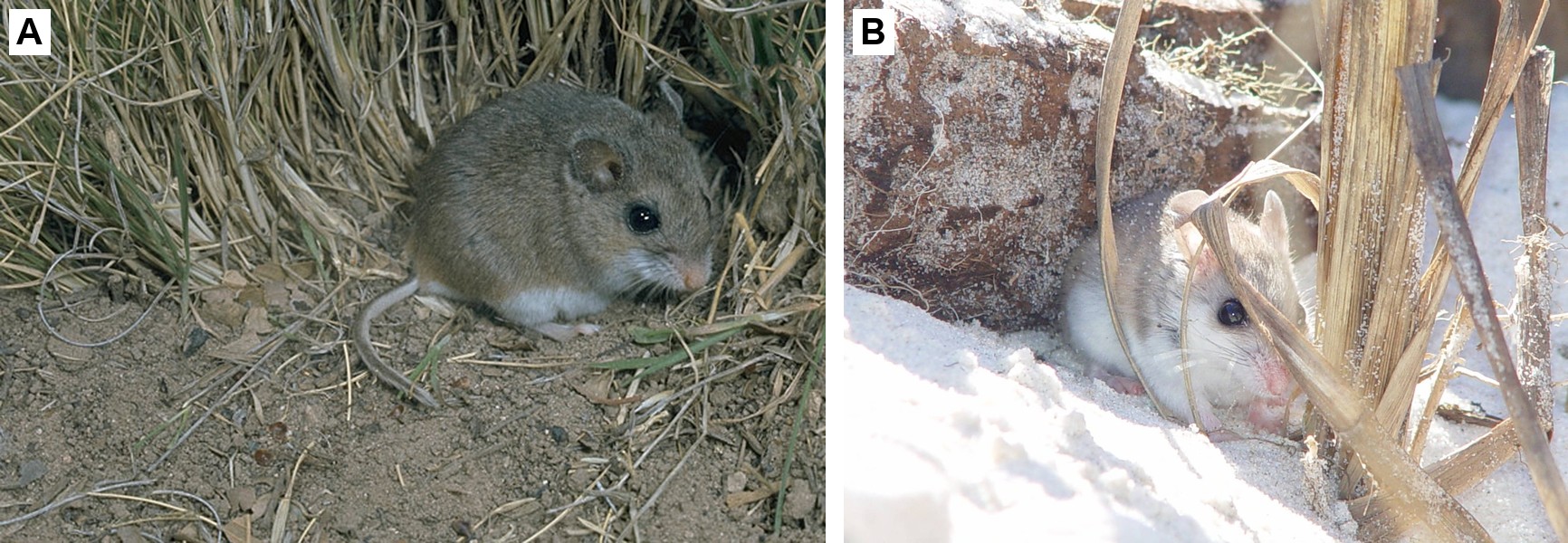
Fig. 15 Same species, different homes. (A) An oldfield mouse (Peromyscus polionotus) of the typical darker inland type, on soil and dry grass. Photo by Roger W. Barbour, U.S. Fish and Wildlife Service, via Wikimedia Commons (public domain). (B) An Alabama beach mouse (P. polionotus ammobates) on white dune sand in the Bon Secour National Wildlife Refuge. Photo by Jackie Isaacs, U.S. Fish and Wildlife Service, via Wikimedia Commons (public domain).

What’s great about this system is that people have nailed down every piece of the story. First, it’s genetic. Hopi Hoekstra and colleagues found that a single amino acid change in a pigmentation gene called Mc1r helps make Gulf coast beach mice lighter, and that new allele is common on the beaches and absent inland (Hoekstra et al. 2006).

Second, it’s adaptive, and they showed it with a clever home-versus-away experiment that is basically a reciprocal transplant. Sacha Vignieri and colleagues made hundreds of clay model mice, some painted light and some painted dark, and set them out on both the beach dunes and in inland fields. Then they counted which models got attacked by predators, mostly birds and mammals hunting by sight. Models that didn’t match their background got attacked way more often than models that did- light models got hit inland and dark models got hit on the beach (Vignieri et al. 2010). So being the right color for your home matters, and it’s predators that are doing the selecting.

Third, and this is the part that connects to our model, gene flow hasn’t erased the difference. Beach and inland populations are connected, and there’s a gradient of mouse color running from the coast inland that tracks how bright the soil is. Lynne Mullen and Hoekstra compared that color cline to neutral genetic markers from the same mice. The neutral markers change only gradually across the region, just like you’d expect from gene flow mixing things up. But mouse color changes much more sharply, right where the soil changes (Mullen and Hoekstra 2008). That’s the signature of selection holding the line against migration. Gene flow is moving alleles back and forth across the whole region, but at the color genes selection is strong enough (\(s > m\)) to keep the beaches pale and the fields dark.

As an instructive exercise go and iterate these equations for some realistic values of \(s\) and \(m\), and check that you land where our equation says you should. (You’ll be really close but maybe not exactly on it, depending on whether you let migration happen before or after selection in each generation. Why would that matter?)