Lecture 9: Genetic Drift

Lecture 9: Genetic Drift¶

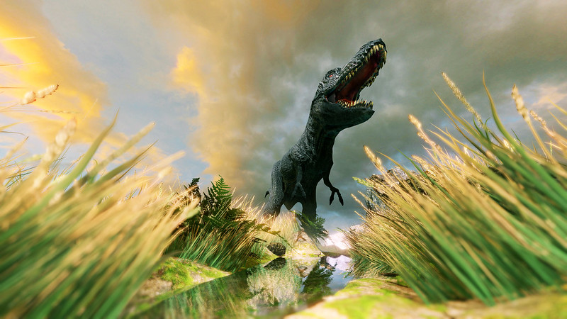
Genetic drift refers to random fluctuations in allele frequencies due to random sampling of alleles in finite populations. The previous lectures have all dealt with deterministic (predictable) evolutionary forces often referred to as linear pressures. Genetic drift is a stochastic (random) force that can scramble the predictable effects of selection, mutation, and gene flow. While it might seem that a random force would be of little significance to evolutionary “progress” (we’ll confront this loaded term later), genetic drift may be an extremely important force in evolution. However, its strength depends on the size of the population, as a simple exercise in coin tossing will illustrate. In ten tosses you might easily get seven heads; in 1000 tosses, however, you would never get 700 heads with a “fair” coin. The same sort of random fluctuation in allele frequencies can occur in small populations: consider a bag full of red and black marbles each in equal frequency; pull out a small handful and the frequency in your hand will probably not equal the frequency in the original bag. Let that handful determine the frequency in a new population. A second small handful will randomly shift the frequency to yet another frequency. If you pulled out all the marbles in the bag (= large population) then the frequency would be maintained exactly in the next generation. Genetic drift is not a potent evolutionary force in very large randomly mating populations. See Fig. 9 for a graphical illustration of this.

Fig. 9 Urn problem captures genetic drift. In this experiment we start with an urn full of red and black marbles at generation 1. We then randomly select marbles, sampling with replacement to form the next generation. Notice how random sampling after 10 generations has substantially changed the frequency of the red marble.¶

Genetic drift: the algorithm¶

Here’s a very simple algorithm that describes all of the essentials of genetic drift. If you already know how to program a computer, a very good exercise would be to code this up. If you don’t know how to program yet, but are interested in learning come find me and I’ll show you a nice way to write this in a simple programing language called R, or really any language you like.

So here’s the algorithm:

Choose an allele at random from the 2N alleles in the parental generation
Make an exact copy of the allele
Place the copy of the allele in the next generation
Go back to 1 until the next generation has 2N alleles

This is exactly the algorithm I used to generate Fig. 9. Can you replicate this figure?

Genetic drift as a dispersive force¶

One of the main ways that genetic drift acts is as a dispersive force on allele frequencies (i.e. it moves allele frequencies about randomly). A neat way to see this is to imagine replicate populations (either experimental or natural). Consider a grid of small populations (e.g., ponds in New Hampshire), all with the same small population size and all starting at time t with $p = q= 0.5$. Through time each population will experience genetic drift due to random sampling and the frequencies in each population will diverge. The distribution of frequencies changes over time from a tight distribution (all 0.5), to a flat distribution (some populations at $p = 0.1$, some at $p=0.9$ and all frequencies in between), to fixation ($p =1.0$) or loss ($p = 0.0$) of the alleles in all populations (think of the Buri experiment). Fixation is when all alleles in the population are $A_1$; this necessarily implies loss of the $A_2$ allele (“fixation” or “loss” should only be used with reference to a specific allele). If each population starts at $p = 0.5$, then at the end, when all populations have lost their variation, 50% of the populations will be fixed for the $A_1$ allele and 50% will be fixed for the $A_2$ allele (latter = “loss” for the $A_1$ allele, get it?). If the initial frequency was $p = 0.7$, then 70% of the populations would be fixed for the $A_1$ allele (again, assuming no selection, migration, mutation).

Main Points: 1) variation lost from within populations but created between replicate populations, 2) alleles fixed or lost from populations due to drift, 3) genetic divergence of populations entirely by chance! No directionality! This implies that evolution cannot be repeated. These are the main ways in which genetic drift can be an important force in evolution of populations with small population size.

Decay in heterozygosity due to drift¶

While studying the full dynamics of genetic drift is difficult mathematically it is simple enough to follow one of the main features of genetic drift, the decay of heterozygosity within populations, through a basic model. Again we turn our attention to our favorite diploid, randomly mating hermaphrodites. We will first describe our population of $N$ diploids by the variable $G$ defined as the probability that two alleles drawn at random from our population are identical by state (e.g. they have the same DNA sequences). Our population is made up of what we call exchangeable or neutral alleles, meaning that alleles are equivalent from the perspective of fitness- no selection is acting. $G$ is very similar to our measure of Homozygosity that we described earlier in the course. When there is no variation in the population $G = 1$, conversely when every allele is unique $G=0$.

We can write down the value of $G$ after one round of random mating and drift, $G'$, as a function of its current value and the population size

\[\begin{aligned} G'= \frac{1}{2N} + \left(1 - \frac{1}{2N} \right )G \end{aligned}\]

This equation spells out in its two terms the mutually exclusive ways in which we can sample two alleles that are identical by state (this is also illustrated graphically in the slides associated with this lecture). One way is to sample two alleles who shared a common ancestor in the generation before. The probability that two alleles share a common ancestor in the previous generation is $1/(2N)$. This is simple enough to understand- given that you’ve chosen one allele, the probability that the next allele has the same parent is just $1/(2N)$ because all parents are equally likely. The second way to sample two alleles that are identical by state is to choose two alleles who don’t share a parent (i.e. $1-1/(2N)$), but who’s parents were themselves identical by state (by definition this probability is $G$). These leaves us with the probability of the second event being $[1-1/(2N)]G$. As the two ways of picking alleles identical by state are mutually exclusive we take the sums of their probabilities and we arrive at $G'$. Nice right?

As is frequent in our population genetic models, I’m going to pull a bit of a bait and switch on you. We just defined the probability of choosing alleles identical by state, but now lets focus on the converse, the probability that you choose two alleles which differ by state. The is both instructive and easier to work with. Define $H$ to be the probability that two randomly sampled allele are different by state (i.e. different DNA sequences), and notice that $H$ is very similar to heterozygosity that we had defined earlier. By definition, $H = 1-G$, which implies that

\[\begin{aligned} H' = 1-G' = \left (1-\frac{1}{2N} \right)H \end{aligned}\]

Now let’s do what comes naturally and look at how $H$ changes per generation. We’ll call this change in heterozygosity $\Delta_NH$ to draw attention to the fact that population size is what’s leading to the change in $H$. So

\[\begin{split}\begin{aligned} \Delta_NH & = & H' - H \\ & = & \left(1 - \frac{1}{2N} \right)H -H \\ & = & -\frac{1}{2N}H \end{aligned}\end{split}\]

Immediately we can see something about how population size should dictate $H$ in finite populations. The probability that two alleles are different by state decreases at a rate $1/(2N)$ per generation. This implies that large populations will lose variation more slowly than small populations due to drift, however they will eventually lose all of their variation.

We can also describe the decay in heterozygosity as a difference equation which captures all of the same dynamics from some initial condition $H_0$ until some time $t$ at which heterozygosity has decreased to $H_t$

\[\begin{aligned} H_t = H_0 \left(1 - \frac{1}{2N} \right)^t \end{aligned}\]

Here we see that the decay in $H$ is geometric. This means that the probability of two alleles being different by state monotonically decreases, however it never reaches exactly zero. As an exercise write down the half-life of heterozygosity using this difference equation, that is solve for the time until $H$ decreases to half it’s original value $H_0/2$.

Fixation Probability of a neutral mutation¶

Quick detour to the world of molecular evolution. If drift means that ultimately alleles are fixed or lost from populations, which allele $A_1$ or $A_2$ gets to fix? Asked another way, what is the probability that an allele will fix in a population? This probability is known as the fixation probability and it has a special place in the world of population genetics and molecular evolution.

Let’s consider our idealized population of $2N$ completely neutral, exchangeable alleles. Lets start with the case when $H=1$ and each allele is unique in the population. We know that this population, like all populations which drift, will eventually go to $H=0$ and in so doing fix an allele. The chance that any particular allele among our $2N$ unique alleles will be that survivor is $1/(2N)$, as they are all exchangeable. If instead there were $i$ copies of some allele, the chance that it would be chosen to fix would be $i/(2N)$. Written another way, if the frequency of $A_1$ is $p$ in a population, then the frequency that $A_1$ fixes is $p$. Thus the probability of fixation of a neutral allele at frequency $p$ in the current population is

\[\begin{aligned} Prob(fix|p) = \pi(p) = p \end{aligned}\]

This probability will play an important role in our study of molecular evolution, but for now just marvel at the symmetry of neutral evolution.

Mutation and Drift¶

Ultimately genetic drift is a force acting to remove variation from populations, so why does genetic variation persist in populations? The answer is of course mutation. Mutations form the raw stuff in evolution, and the balance between mutation and drift will occupy our attention when we study molecular evolution. The Neutral Theory of Molecular Evolution, formalized by Motoo Kimura, says that main the forces acting on populations are drift and mutation, and that DNA sequence differences between individuals and species are mostly neutral mutations. Here will develop the mathematical models which underlie neutral variation within species

First we’ll turn our attention back to $G$, the probability that two alleles are identical by state (i.e. have the same DNA sequence). The value of $G$ after one round of drift and mutation as a function of its current value is

\[\begin{aligned} G' = (1-u)^2\left [ \frac{1}{2N} + \left(1 - \frac{1}{2N} \right )G \right]. \end{aligned}\]

Let’s look at this for a moment. You’ll notice that the only thing that differs with our addition of mutation is the term $(1-u)^2$. This term represents the probability that no mutations occurred in either of the alleles we sampled ($(1-u)$ is the probability that no mutation occurred in one of the alleles).

Now let’s try to poke at $G'$ until we can obtain an expression for $\Delta_{N,u}H$, the change in heterozygosity due to drift and mutation. This will allow us to write down an equilibrium solution for $\hat{H}$ that will tell us something about what the heterozygosity of populations should be in nature. Using that fact that mutation rate, $u$, is small and that population size, $N$, is in comparison large, we can approximate $G'$. We will assume that we can ignore terms with $u/N$ as a factor and will approximate $(1-u)^2$ with $(1-2u)$

\[\begin{split}\begin{aligned} G' & \approx & (1-2u) \left [ \frac{1}{2N} + \left(1 - \frac{1}{2N} \right )G \right] \\ & \approx & \frac{1}{2N} + \left ( 1 - \frac{1}{2N} \right )G - 2uG \end{aligned}\end{split}\]

Now lets make the switch to heterozygosity using $H = 1-G$ and rearranging to get

\[\begin{aligned} H' \approx \left( 1 - \frac{1}{2N} \right ) H + 2u(1-H). \end{aligned}\]

Now the change in $H$ in any generation is $$\Delta_{N,u}H = H' -H$$,

\[\begin{aligned} \Delta_{N,u}H = - \frac{1}{2N}H + 2u(1-H) \end{aligned}\]

and at equilibrium $\Delta_{N,u}H = 0$ and after a tiny bit of algebra

\[\begin{aligned} \hat{H} = \frac{4Nu}{1+4Nu} \end{aligned}\]

That’s what we’re after- a simple expression that relates heterozygosity to mutation rate and population size. The compound parameter $4Nu$ plays an important role in population genetics. This can be seen clearly here. When $4Nu$ is large, mutation dominates drift and populations retain genetic variation. When $4Nu$ is small, drift dominates and genetic variation is driven out of populations. Fig. 10 shows this relationship graphically.

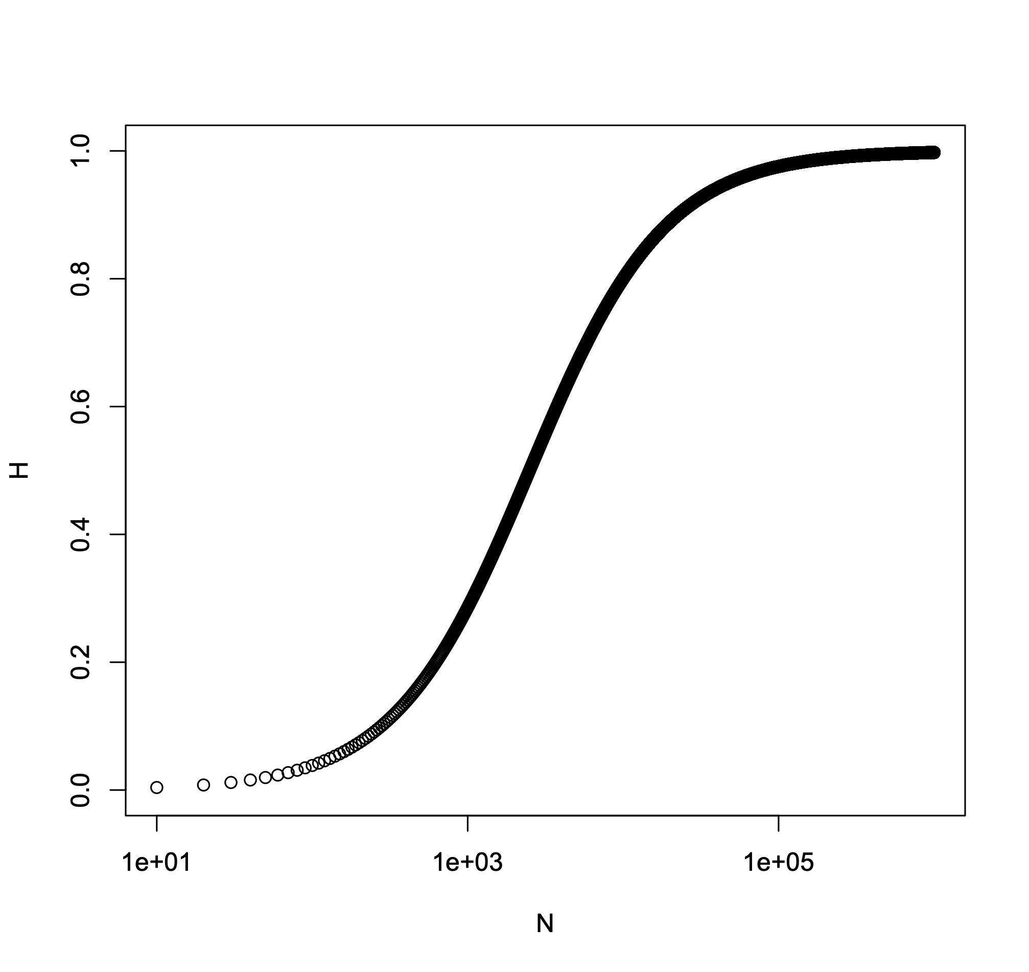
Fig. 10 Heterozygosity as a function of $N$. Expected heterozygosity under drift and mutation is shown as a function of $N$, where $u=10^4$ is held constant.¶

Effective population size¶

In neutral populations, we can describe the rate at which the populations drifts by its size. Our population however is an idealized population of random mating hermaphrodites that remain at constant population size. This describes only a very small portion of real populations though.

Multiple factors can cause populations to drift faster then their population size would predict. These include unequal sex ratios, changes in population size, variance in reproductive success, and inbreeding. When these things occur we describe the population by its effective population size, or the size that it would have to be for drift to proceed at its observed rate.

Let’s look at changes in population size first. If a population goes through $i$ epochs at population size $N_i$, then the effective population size of the population is given by the harmonic average of the populations sizes

\[\begin{aligned} N_e= \frac{n}{\sum_{i=1}^{n}\frac{1}{N_{i}}} < \frac{1}{n} \sum_{i=1}^{n}N_{i} \end{aligned}\]

The harmonic average is always smaller than the arithmetic average. This implies that periods of time in which a population is at small size disproportionally affect rates of genetic drift.

If populations have unequal sex ratios among breeding individuals then again $N_e$ is modified. For example imagine the case of sea lions in which males guard a harem of females. Many fewer males get to breed in any generation than females which changes the effective number of alleles in a population. The relation that describes this effect is seen below.

$$\begin{aligned} N_e= \frac{4N_m N_f}{N_m + N_f} \end{aligned}$$ Take a look at the

magnitude of $N_e$ reduction in this equation versus the one we arrived at for changes in effective population size. Which do you think is more important over evolutionary time?

Lecture 8: Mutation, Migration, with and without selection

Lecture 10: Evolution as a combination of forces

Bio 380-- Evolutionary Biology