
Lecture 22: Genetics of speciation
Contents
Lecture 22: Genetics of speciation
Speciation has occurred, is occurring and will occur. These are undeniable facts. The problem is: How do we study speciation? There is no single approach since there is no single mechanism by which species speciate. Some approaches used in the past: Study patterns of morphological change in the fossil record in a well defined lineage of organisms. Success depends on many unknowns: stratigraphic resolution (will you “see” the speciation event); distinguishing geographic variants from true species (all you have is morphology. Comparisons of closely related species. These have speciated recently (assuming closely related short time since speciation) so careful studies of their biology may identify important features that contribute to reproductive isolation.
Study intraspecific variation. Look for evidence of incipient barriers to gene exchange. Perform crosses between individuals from different regions; look for differences in genital morphology, secondary sexual characteristics. These may show some bimodal distribution suggestive of early steps in evolution. Must ask: what might we expect to find? This depends entirely on the model of speciation that might apply to the organism under study. Looking within a large species range for signs of variation may be fruitless if the speciation mode is peripatric with genetic revolutions?
Measuring speciation at the genetic level
Laboratory populations might serve as model systems. One can establish the conditions of the specific model under question and ask if the predicted divergence is observed. Mathematical models can address specific predictions about modes of speciation. Both of these “artificial” methods are important since they can identify what is possible. Knowing what’s possible might spur one on to looking for it in unexpected contexts in natural populations. With the use of molecular tools the comparisons of intraspecific and interspecific genetic variation has been studied in some detail. Aim is to identify genetic changes during speciation. These data show us that genetic change is associated with speciation. We want to be able to describe the genetics of speciation and the genetics of species differences. To do so we need to distinguish genetic changes that cause speciation from those that accompany speciation. These will differ a lot from one group of organisms to the next and will depend on the genetic architecture of speciation. Best data on both of these issues have come from the many species of Drosophila. Ayala took early step looking at genetic differentiation across populations, sub-species, semi-species, and full species. Found that full species at larger genetic distances than did say sub populations, as you might expect. Coyne and Orr (1989, Evolution vol. 43, pg. 362-381) take Ayala’s approach one step further and attempt to correlate genetic distance with amounts of prezygotic and postzygotic isolation. In the literature there are many reports of the amount of genetic distance between closely related species of Drosophila and the amount of reproductive isolation between many of the species for which genetic distance has been measured (premating or prezygotic isolation is measured as [1-(proportion of heterotypic matings/proportion of homotypic matings)] which ranges from - infinity for all heterotypic (between species) matings to 0 for random mating to +1 for all homotypic matings. Rarely do two species prefer to mate with the wrong type so the index effectively ranges from 0 to 1). Postzygotic or postmating isolation can be measured as in the following example. Consider two species, A and B. These can be crossed two ways (reciprocally) to produce hybrid offspring. We can also examine the viability or fertility of the two sexes of these hybrid offspring, hence four contexts are examined to score postzygotic isolation:
Case |
Female parent |
Male parent |
Offspring |
Inviable or sterile? |
|---|---|---|---|---|
1 |
Species A |
Species B |
Male |
Yes = 1 |
2 |
Species A |
Species B |
Female |
No = 0 |
3 |
Species B |
Species A |
Male |
No = 0 |
4 |
Species B |
Species A |
Female |
No = 0 |
We then define the isolation index (\(I\)) to be equal to the average score of the four cases- in this example \(I=0.25\). In any particular case one could choose to score isolation in terms of the presence or absence of either isolation or sterility. Normally hybrid sterility evolves before hybrid inviability (mules are sterile but viable). Hence an index based on sterility would have higher values than an index based only on evidence for inviable hybrid offspring.
Coyne and Orr extracted these two types of data from the literature and tested some important ideas about the genetics of speciation. The general idea is that genetic distance (D) is positively related to time (the molecular clock hypothesis) and thus species pairs showing different degrees of genetic distance should be at different degrees of completion of the speciation process (be aware that many organisms are in the process of speciating as you read these notes). Coyne and Orr show that there is a significant relationship between genetic distance and both premating and postmating isolation Two interesting additional points: sympatric species show greater prezygotic isolation than allopatric species pairs. This pattern is consistent with the reinforcement hypothesis and suggest that reinforcement can act.
A second observation: less genetic distance between species pairs that produce sterile or inviable males than between species pairs that produce sterile or inviable females.
Haldane’s Rule
Coyne and Orr’s (1989) second observation confirmed a well documented pattern known as Haldane’s Rule stating that when hybrid crosses produce sterile or inviable offspring, the sex that exhibits this is most likely the heterogametic sex (the sex with two different sex chromosomes, e.g. X and Y in male humans and Drosophila; in birds and butterflies the female is heterogametic with Z and W). Another “rule” of speciation is that genes affecting reproductive isolation are typically found on the X chromosome (where X is the “female” chromosome; see another paper by Coyne and Orr: “Two Rules of Speciation”, in Speciation and its Consequences, 1989, D. Otte & J. Endler, editors, Sinauer Associates). Muller first proposed X-effect as explanation for Haldane’s rule. Basic idea is that X-linked incompatibilities which are recessive will be exposed in males (heterogametic sex), and thus be more likely to lead to male inviability or sterility. When individuals are crossed between divergent populations, there will deleterious pleitropic interaction effects between these new alleles on the X and other genes throughout the genome. The new mutations certainly were not deleterious when they arose within each separated population, but when paired with autosomes from a diverged population these mutations do not function properly, thus one would only see the effect in a hybrid cross.
Dobzhansky-Muller model
The Dobzhansky-Muller model of genic incompatibility in speciation leads to a general explanation of Haldane’s rule and the X-effect on male hybrids. We imagine a population that is currently fixed at two loci for aabb. We imagine that this population splits in to two, and each daughter population diverges genetically (see Figure 1)
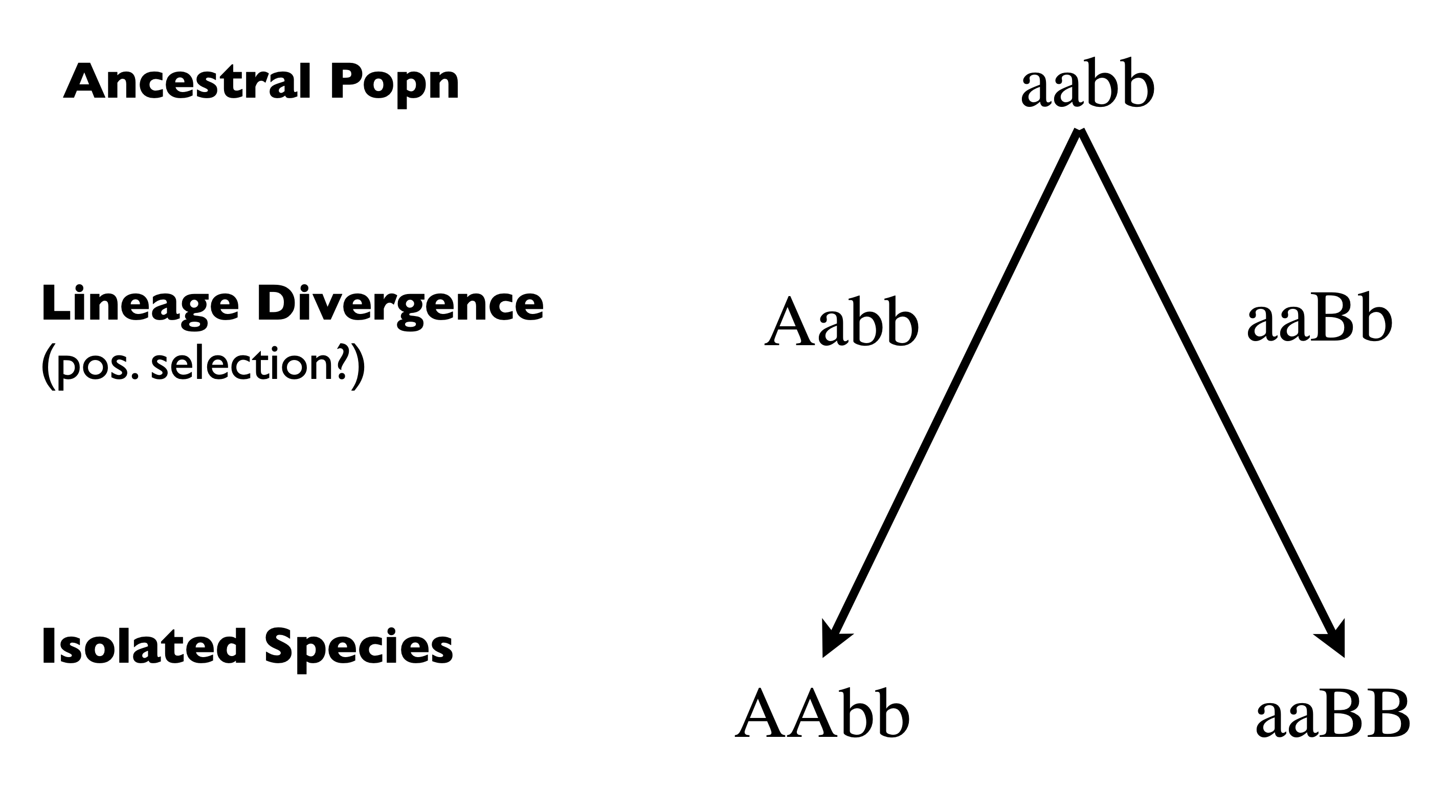
Fig. 20 Dobzhansky-Muller model of the evolution of postzygotic isolation An ancestral population is fixed for the aabb genotype. It splits in to two daughter lineages each of whom fixes a novel allele at an interacting locus. When hybrids from the daughter lineages are formed the A allele interacts with the B allele to cause fitness loss in the hybrid
This model predicts that you need substitutions at both loci for incompatibility, that incompatibilities could indeed be asymmetric between species, and that the number of incompatibilities in a lineage should increase faster than linear with time.
Finding Dobzhansky-Muller interactions
Attempts to identify genes that keep species isolated go back to Dobzhansky in the 1930’s: crosses between D. pseudoobscura and D. persimilis produce sterile males and fertile females as F1 hybrids. These F1 females can be backcrossed to males of either species, so the backcrossed offspring can have all combinations of chromosomes. With four chromosome pairs in each species, the F1 hybrid will have four heterokaryotypic pairs of chromosomes. The two possible backcrosses (one in each direction) can result in 16 possible combinations of chromosomes. Frequently find that the offspring with nonmotile sperm (= sterile) are the ones with sex chromosomes from each species (see figures). Deleterious interactions between sex chromosomes and/or between sex chromosomes and autosomes are implied, but the details are the topic of a lot of current research (see Orr 1993, Nature vol. 361, pg. 532 & pg. 496). These types of experiments, coupled with molecular biology may someday allow us to identify the genes and the types of changes that can lead to speciation. Again, we would like to know the genetic architecture of speciation: how many genes involved?; what sorts of mutations at each gene? what sorts of interactions among genes? etc.
Genes of speciation
We are now starting to get our first glimpses of the genetic changes that cause postzygotic isolation among species – sometimes there are called speciation genes (a terrible name if you think about it long enough). Basic idea is to try to map incompatibilities between species at the genetic level. Some famous examples from Drosophila: Hmr (e.g. Barbash et al. 2000), nup96 (Presegraves et al. 2004). The extraordinary pattern thus far is that the genes themselves are not extraordinary- normal proteins, doing normal protein business (e.g. nup96 is a nuclear pore complex protein), but due to divergence cause “poisonous” interactions which reduce fitness of hybrids. The other pattern- isolation genes evolve quickly between species. This makes intuitive sense given the Dobzhansky-Muller model.