
Lecture 12: Molecular Evolution
Contents
Lecture 12: Molecular Evolution
So far we’ve focused mainly on the impact of evolutionary forces on patterns of genetic variation within populations and species. Now lets shift our attention to how those forces translate to genetic and genomic differences between species.
Rates of Molecular Evolution
The basic quantity in the study of molecular evolution is sequence divergence, or the number of differences between two species at some locus. The basic “work flow” for this kind of study goes something like this
Sequence some locus out of two species (e.g. CFTR from a human and from a chimp)
Align those sequences (this is actually a technical process, but the basic idea is to find molecular homology)
Count the number of differences between sequences in the alignment
This count of the number of differences will be the raw data. Conventionally, the next thing that is done is to express the number of differences on a per site basis. This gets us to a quantity most often called sequence divergence. This isn’t of course necessary, but it is convenient as some loci are bigger than others, thus normalization on the basis of the individual site allows one to come levels of sequence divergence from different genes or different portions of the genome.
As an example lets consider an an amino acid alignment of mammalian sequences from a locus known as FOXP2 (Fig. 13) This alignment consist of 716 amino acid residues from human, chimp, gorilla, orangutan, rhesus macaque, and a mouse outgroup. Let’s focus our attention to human-chimp differences specifically. In this alignment we see 2 simple amino acid differences and one possible insertion/deletion difference. We’ll ignore the insertion/deletion difference for the remainder of this analysis; this is actually common practice in molecular evolution studies, can you figure out why?
If we assume that humans and chimps diverged (i.e. became separate species) from one another approximately 5 million years ago and that there were 2 substitutions along the two lineages in that time, then the rate of substitution at the FOXP2 locus is
We need to multiply by two because each of our substitutions might have taken place on either the lineage leading to humans or the lineage leading to chimps. We of course could use the multiple alignment data in Figure 1 to reconstruct ancestral states, and figure out along which lineage those differences were most likely to occur, but we’ll ignore that complexity for now.
It’s often convenient to express rates of substitution on a per site basis. This allows us to simply compare rates at different loci, or in different portions of the genome. In this case we have aligned 716 aa sites, so our per site calculation is
Believe it or not this is a pretty typical rate of protein evolution. As we proceed into this next section be careful about units- we’ll be developing a simple theoretical model as to what rates of substitution should be that are based on generations as the unit time and not years. This can actually lead to a surprising amount of confusion (even among “professionals”!) so let’s be sure to get everything straight.
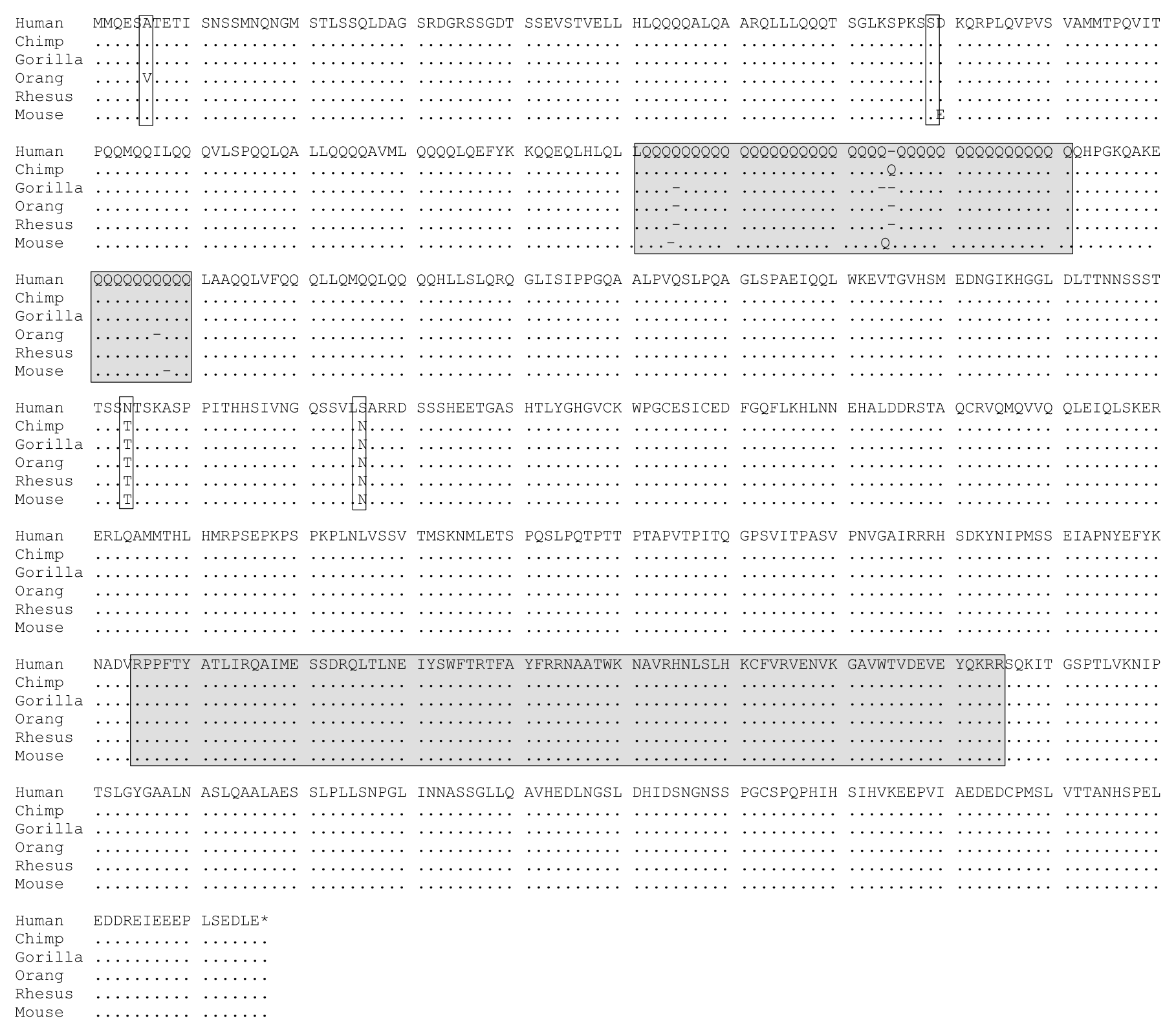
Fig. 13 Multiple Alignment of the FOXP2 gene. 6 mammalian amino acid sequences of the FOXP2 locus are shown. 716 aa sites are represented. We can see 2 simple amino acid differences between human and chimp in this alignment and 1 insertion/deletion difference. This figure is adapted from Enard et al. (2002).
Consider a finite, diploid population that evolves only due to drift and mutation. Substitutions will occur in this population because some fraction of the mutations which enter the population every generation will ultimately drift to frequency one, thus fixing in the population. Thus intuitively we should see that the rate of substitution will be a function of the mutation rate and the population size.
Let’s define \(u\) to be our probability of mutation per gamete per generation. If there are \(2N\) gametes produced in our population each generation that on average we should have \(2Nu\) mutations. In larger populations we should have more mutations entering each generation, and conversely smaller populations should have less mutational input if we hold \(u\) to be fixed. Naively we might then expect evolution (i.e. substitution) to proceed faster in larger populations, and this is true in some contexts, but not in our purely neutral population.
Under neutrality, each of our \(2Nu\) new mutations should be equally likely to fix. As we have proven early, the probability of any of those mutations fixing is simply equal to its frequency, which for new mutations in a diploid population is \(1/(2N)\). We are now ready to calculate the rate of substitution in our neutral population. The rate of substitution should be equal to the number of new mutations entering the population each generation times the probability that each of them fix. That is
So the substitution rate of our neutral population is just equal to the mutation rate. This is an amazing result from population genetics which at first blush is counterintuitive. Shouldn’t fixation that are the result of drift be dependent on population size? Well the symmetry of the situation is such that population size also determines the mutational input of the population, canceling out the dependence of the probability of fixation on population size so that the flux of fixations is only dependent upon the rate of mutation. Truly incredible!
Motoo Kimura, considered the founder of the Neutral Theory of Molecular Evolution, along with Tomoko Ohta put this theoretical prediction to the test by looking at rates of protein evolution over mammalian evolution. What they found was that rates of protein evolution per amino acid site per year were constant enough (\(\approx 10^-9\)) that indeed all substitutions might be neutral. There were many problems with their famous analysis, but perhaps the most glaring was that their unit of time- why should mutation rates be constant across mammalian lineages on a per year basis? The short answer is they shouldn’t- our derivation pertains to mutations per generation, thus we expect a priori that under the neutral model substitution rates should depend on generation times. Ohta did get back to this flaw later, but we unfortunately won’t have time to cover her further work (come take my advanced class if you’re interested).
Once Kimura and Ohta published their result, numerous researchers were up in arms- of course there are differences in rates of evolution among genes or portions of the genome! They would expect them do to different levels of functional constraint. The notion of purifying selection was dear to the proponents of the classical school of genetic variation (e.g. Muller), so how does constraint fit in to the Kimura and Ohta model. Really it’s no problem for the neutral model. Imagine that some fraction of mutations \(f_0\) is purely neutral, and some other fraction \(1-f_0\) is strongly deleterious. If this is the case then that strongly deleterious fraction should never participate in molecular evolution and we have a quick fix to our model, namely
Now different rates of evolution can be explained purely as a function of differing levels of constraint. More constraint leads to a lower fraction of purely neutral mutations (i.e. smaller \(f_0\)) and thus slower rates of evolution. Conversely loci which have little or no functional constraint should be expected to evolve more quickly.
This simple fix is all well and good but do we really believe that mutations are either strongly deleterious or neutral as Muller might have? What about beneficial mutations? Shouldn’t we be including those in our model? Use your biological intuition here- what kinds of mutations should participate in molecular evolution and eventually lead to fixations between species? This is a central question to the study of evolutionary genetics…
Ask yourself this- what should the probability of fixation of a beneficial or deleterious mutation be in relation to a neutral one? Without getting in to the mathematics lets gain a qualitative understanding of how rates of evolution change as a function of the kinds of mutations that enter populations. Fig. 14 shows the expected rates for these alternative models in comparison to the neutral rate. This intuition leads to simple tests of the neutral model based on rates of substitution- how would you go about asking if a gene was evolving under say positive selection?
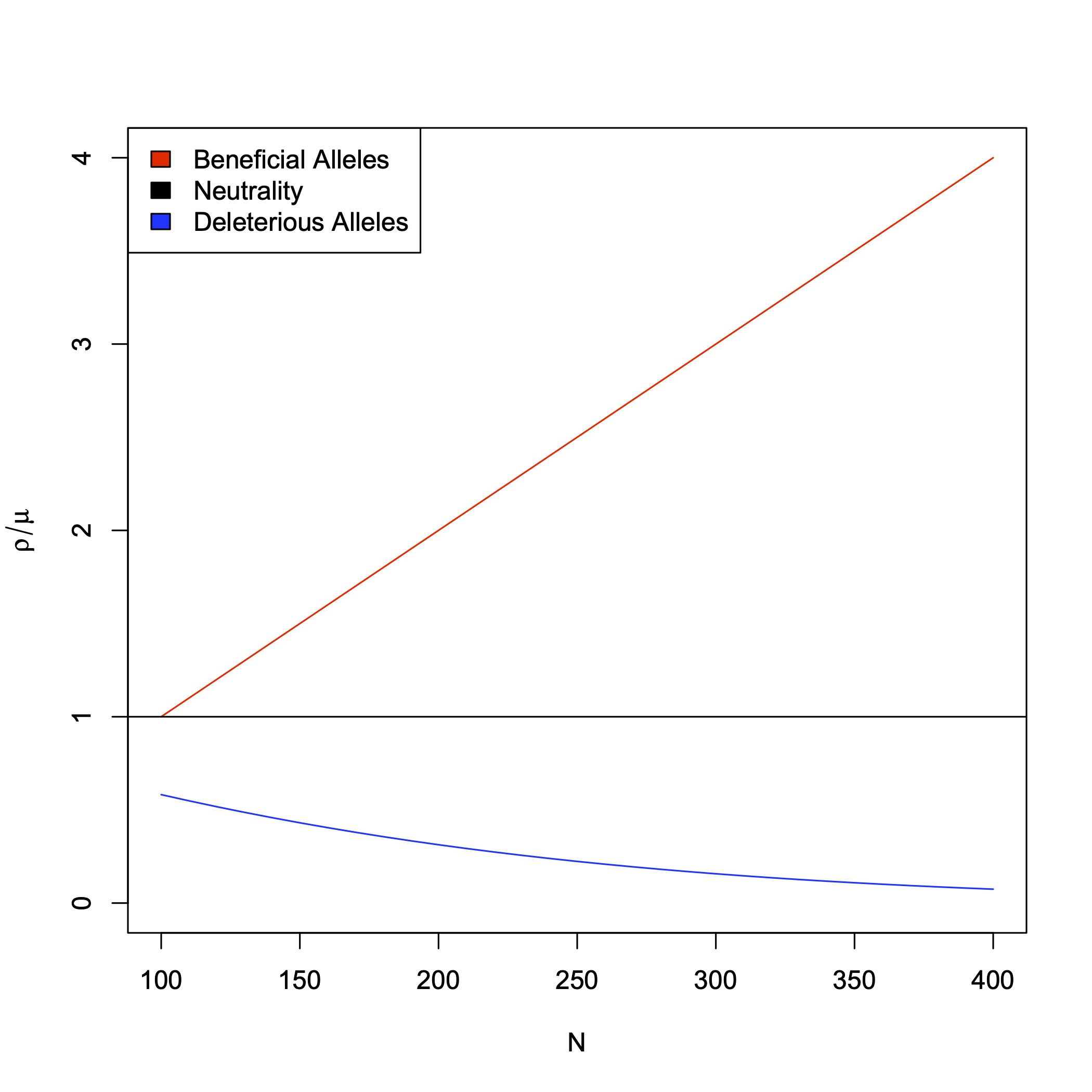
Fig. 14 Rates of substitution. Here we consider rates of substitution for three models, a beneficial alleles model (i.e. Positive Selection) in red, the neutral model in black, and a deleterious allele model (i.e. Purifying selection) in blue. Rates are shown as a function of population size, \(N\), and are normalized by the mutation rate. The the Neutral rate is constant at 1.
Molecular Clocks
Most discussions of the rates of DNA evolution have been with respect to the molecular clock hypothesis which states that there is a positive linear relationship between time since two species diverged and amount of genetic divergence (e.g., DNA sequence difference) between those species - basically Kimura and Ohta’s observation. The fact that genes evolve at different rates indicate that there is not one molecular clock but probably many molecular clocks that “tick” at different rates, and in fact that those “ticks” might increase or decrease in rate over time.
Lets say we could identify a reliable molecular clock (e.g., number of amino acid substitutions in the cytochrome C gene), we can in principle use this to date, or corroborate, evolutionary events of interest (e.g., the divergence times for species that do not have good fossil data). For example: we know that there are \(K_{xy}\) substitutions between species \(x\) and \(y\) and we know that they diverged \(T\)years ago (from fossil data). Thus the rate of molecular evolution is \(r = K{xy}/2T\). Now lets say we obtain the sequence of cytochrome C from 3 other species \(a\), \(b\) and \(c\). If we wanted to known their divergence times, we could assume that the molecular clock that we had calibrated using the the \(x\) to \(y\) comparison should apply and back calculate divergence times simple from levels of genetic divergence between our other species. In my humble opinion this approach has major short comings- what are they?
Polymorphism and Divergence
One of the nicest features of the neutral model is that it predicts a correlation in levels of polymorphism within populations and divergence between species. Briefly lets examine why this is so. We said already that the rate of substitution at neutral loci is purely dependent on the rate of mutation. That is \(\rho=u\). Recall from our work on equilibrium expectations of heterozygosity that we came up with an expression for heterozygosity in neutral populations that depended on a joint parameter of population size and mutation rate, \(4Nu\). If we call this joint parameter \(\theta = 4Nu\), then we can rewrite our simple expression for equilibrium heterozygosity as
As levels of heterozygosity are going to depend on \(\theta\) alone its of great interest to try to estimate this parameter out of real data. Accordingly there are numerous ways to estimate \(\theta\), including just doing what comes naturally and summing up the expected frequency of heterozygotes from allele frequencies in a population.
Let’s step back quickly and look at what we have here. Rates of substitution will depend on \(u\) where as levels of heterozygosity will depend on both \(u\) and \(N\) through \(\theta\), thus under neutrality we should have a simple correlation between levels at diversity at a locus and it’s rate of substitution. Again this could lead to tests of the neutral model of molecular evolution- can you figure out how that might work?
Perhaps the simplest test of the neutral model which uses both polymorphism and divergence is the McDonald-Kreitman test (or MK test). The MK test compares the number of mutations which are polymorphic (i.e. segregating within a population) to the number of mutations which are fixed (i.e. contributing to divergence) between species at two loci, one that should be neutral and one that might be under selection (the classic example is synonymous sites versus non-synonymous sites). Call the number of polymorphisms at synonymous sites and non-synonymous sites \(P_s\) and \(P_n\) respectively. Similarly call the number of fixed differences \(D_s\) and \(D_n\). Now lets imagine that each of our two sites had different rates of mutation, \(u_s\) and \(u_n\). Under the neutral model \(P_s\) should be proportional to \(4Nu_s\) and and \(D_s\) should be equal to \(u_s\). The same should be true for non-synonymous sites, that is \(P_n \propto 4Nu_n\) and \(D_n = u_n\). Now consider the ratio of polymorphism to divergence at each of our loci. Under neutrality
Thus if these ratios are not equal the neutral model can be rejected. This is a powerful test of the neutral model and one that is very population in modern evolutionary genomics.
Perhaps more than any other innovation in population genetics, this expected correlation between polymorphism and divergence has had great explanatory power in understanding patterns of genomic variation. For example- why do regions of low recombination show less variation than regions of normal recombination? This pattern, which has been observed in everything from corn and pine trees, to fruit flies and humans can only be understood in light of the mechanisms we have talked about.